- Sumit Dey
- Mar 7, 2022
- 7 min read
Updated: Mar 10, 2022
This part is the continuation of Computer Vision and Convolutional Neural Networks(CNN) with TensorFlow(Part 1)
In our previous part model works with two classes(pizza and steak), in this section, we would work on 10 different image classes.
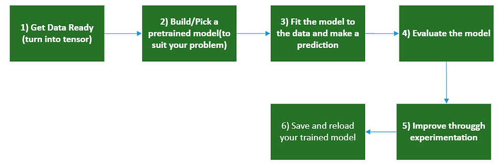
How about we go through those steps again, except this time, we'll work with 10 different types of food.
Become one with the data (visualize, visualize, visualize...)
Preprocess the data (prepare it for a model)
Create a model (start with a baseline) Fit the model
Evaluate the model
Adjust different parameters and improve the model (try to beat your baseline)
Repeat until satisfied.
Import Data
we've got a subset of the Food101 dataset. In addition to the pizza and steak images, we've pulled out another eight classes.
import zipfile
# Download zip file of 10_food_classes images
# See how this data was created - https://github.com/mrdbourke/tensorflow-deep-learning/blob/main/extras/image_data_modification.ipynb
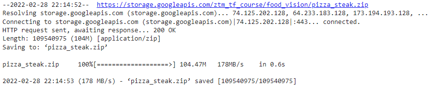
!wget https://storage.googleapis.com/ztm_tf_course/food_vision/10_food_classes_all_data.zip
# Unzip the downloaded file
zip_ref = zipfile.ZipFile("10_food_classes_all_data.zip", "r")
zip_ref.extractall()
zip_ref.close()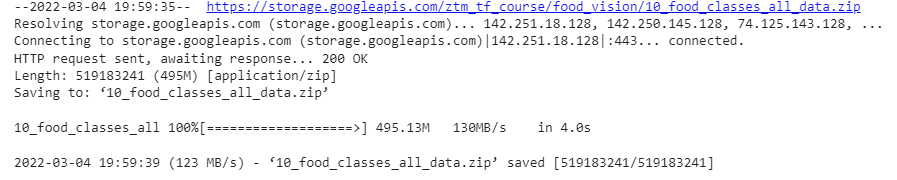
Let's see the different directories and sub-directories of 10_food_classes files
import os
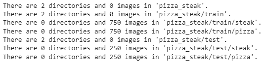
# Walk through 10_food_classes directory and list number of files
for dirpath, dirnames, filenames in os.walk("10_food_classes_all_data"):
print(f"There are {len(dirnames)} directories and {len(filenames)} images in '{dirpath}'.")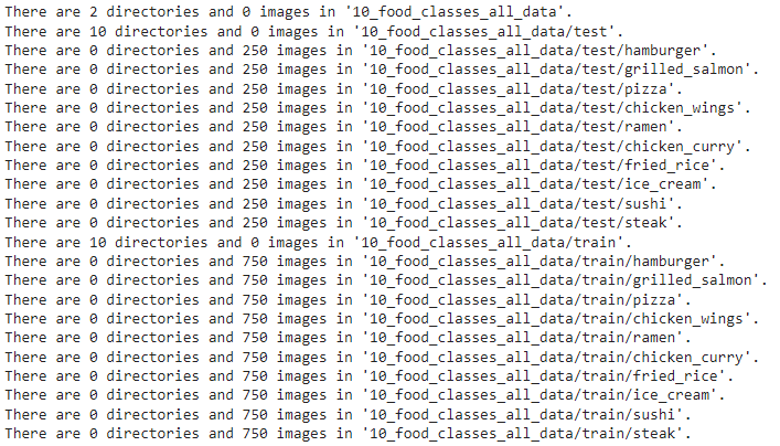
Let's find out the class names from the subdirectories
train_dir = "10_food_classes_all_data/train/"
test_dir = "10_food_classes_all_data/test/"
import pathlib
import numpy as np
data_dir = pathlib.Path(train_dir)
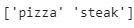
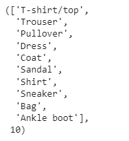
class_names = np.array(sorted([item.name for item in data_dir.glob('*')]))
print(class_names)
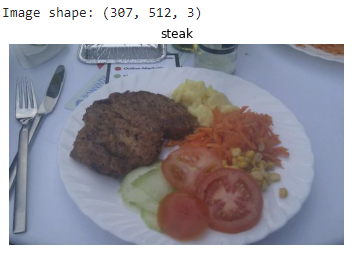
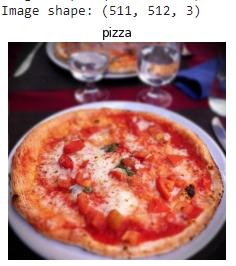
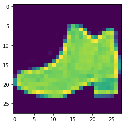
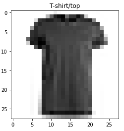
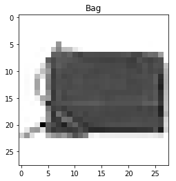
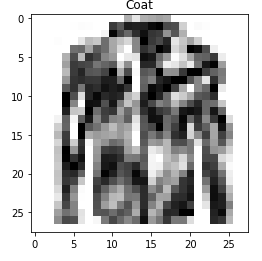
Let's visualize an image from the training set
# View a random image from the training dataset
import random
img = view_random_image(target_dir=train_dir,
                        target_class=random.choice(class_names)) # get a random class name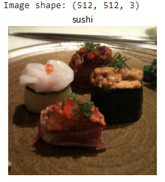
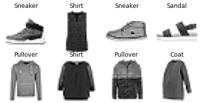
We can try for more images.
Preprocessed the data(prepare for the model)
Time to preprocess the data using ImageDataGenerator
from tensorflow.keras.preprocessing.image import ImageDataGenerator

# Rescale the data and create data generator instances
train_datagen = ImageDataGenerator(rescale=1/255.)
test_datagen = ImageDataGenerator(rescale=1/255.)

# Load data in from directories and turn it into batches
train_data = train_datagen.flow_from_directory(train_dir,
                                               target_size=(224, 224),
                                               batch_size=32,
                                               class_mode='categorical') # changed to categorical

test_data = train_datagen.flow_from_directory(test_dir,
                                              target_size=(224, 224),
                                              batch_size=32,
                                              class_mode='categorical')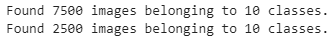
As with binary classification, we've creator image generators. The main change this time is that we've changed the class_mode parameter to 'categorical' because we're dealing with 10 classes of food images, everything else remains the same.
Now question Why is the image size 224x224? This could actually be any size we wanted, however, 224x224 is a very common size for preprocessing images to. Depending on your problem you might want to use larger or smaller images.
Create a baseline model
We can use the same model we used for the binary classification problem, now for the multi-class classification problem with a couple of small tweaks.
Changing the output layer to use have 10 ouput neurons (the same number as the number of classes we have).
Changing the output layer to use 'softmax' activation instead of 'sigmoid' activation.
Changing the loss function to be 'categorical_crossentropy' instead of 'binary_crossentropy'.
import tensorflow as tf
from tensorflow.keras.models import Sequential
from tensorflow.keras.layers import Conv2D, MaxPool2D, Flatten, Dense

# Create our model (a clone of model_, except to be multi-class)
model_baseline = Sequential([
  Conv2D(10, 3, activation='relu', input_shape=(224, 224, 3)),
  Conv2D(10, 3, activation='relu'),
  MaxPool2D(),
  Conv2D(10, 3, activation='relu'),
  Conv2D(10, 3, activation='relu'),
  MaxPool2D(),
  Flatten(),
  Dense(10, activation='softmax') # changed to have 10 neurons (same as number of classes) and 'softmax' activation
])

# Compile the model
model_baseline.compile(loss="categorical_crossentropy", # changed to categorical_crossentropy
                optimizer=tf.keras.optimizers.Adam(),
                metrics=["accuracy"])
Fit the baseline model
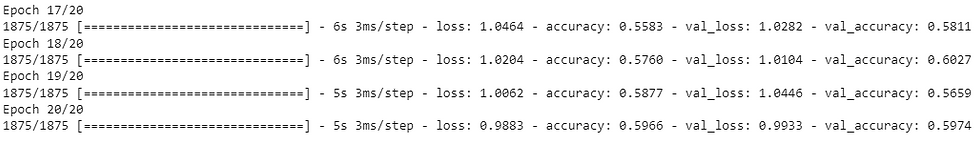
# Fit the model
history_baseline= model_baseline.fit(train_data, # now 10 different classes
                        epochs=5,
                        steps_per_epoch=len(train_data),
                        validation_data=test_data,
                        validation_steps=len(test_data))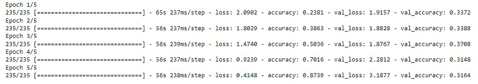
Why do you think each epoch takes longer than when working with only two classes of images?
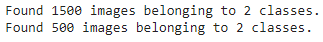
It's because we're now dealing with more images than we were before. We've got 10 classes with 750 training images and 250 validation images each totaling 10,000 images. Whereas when we had two classes, we had 1500 training images and 500 validation images, totaling 2000.
The intuitive reasoning here is the more data you have, the longer a model will take to find patterns.
Evaluate the model
We've just trained a model on 10 different classes of food images, let's see how it went.
# Evaluate on the test data
model_baseline.evaluate(test_data)
Check out the model's loss curves on the 10 classes
# Check out the model's loss curves on the 10 classes of data
plot_loss_curves(history_baseline)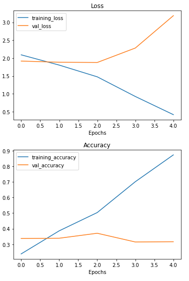
That's quite the gap between the training and validation loss curves.
What does this tell us? It seems our model is overfitting the training set quite badly. In other words, it's getting great results on the training data but fails to generalize well to unseen data and performs poorly on the test data.
Adjust the model parameters
Due to its performance on the training data, it's clear our model is learning something. However, performing well on the training data is like going well in the classroom but failing to use your skills in real life.
Ideally, we'd like our model to perform as well on the test data as it does on the training data.
So our next steps will be to try and prevent our model overfitting. A couple of ways to prevent overfitting include:
Get more data - Having more data gives the model more opportunities to learn patterns, patterns that may be more generalizable to new examples.
Simplify model - If the current model is already overfitting the training data, it may be too complicated of a model. This means it's learning the patterns of the data too well and isn't able to generalize well to unseen data. One way to simplify a model is to reduce the number of layers it uses or to reduce the number of hidden units in each layer.
Use data augmentation - Data augmentation manipulates the training data in a way that's harder for the model to learn as it artificially adds more variety to the data. If a model is able to learn patterns in augmented data, the model may be able to generalize better to unseen data.
Use transfer learning - Transfer learning involves leveraging the patterns (also called pre-trained weights) one model has learned to use as the foundation for your own task. In our case, we could use one computer vision model pre-trained on a large variety of images and then tweak it slightly to be more specialized for food images.
If you've already got an existing dataset, you're probably most likely to try one or a combination of the last three above options first.
Since collecting more data would involve us manually taking more images of food, let's try the ones we can do from right within the notebook.
Let's simplify our model, To do so, we'll remove two of the convolutional layers, taking the total number of convolutional layers from four to two.
# Try a simplified model (removed two layers)
model_improve = Sequential([
  Conv2D(10, 3, activation='relu', input_shape=(224, 224, 3)),
  MaxPool2D(),
  Conv2D(10, 3, activation='relu'),
  MaxPool2D(),
  Flatten(),
  Dense(10, activation='softmax')
])

model_improve.compile(loss='categorical_crossentropy',
                 optimizer=tf.keras.optimizers.Adam(),
                 metrics=['accuracy'])

history_improve = model_improve.fit(train_data,
                          epochs=5,
                          steps_per_epoch=len(train_data),
                          validation_data=test_data,
                          validation_steps=len(test_data))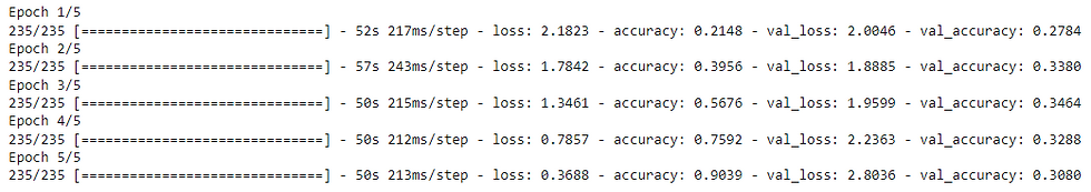
Let's check out the loss curves
# Check out the loss curves of model_improve
plot_loss_curves(history_improve)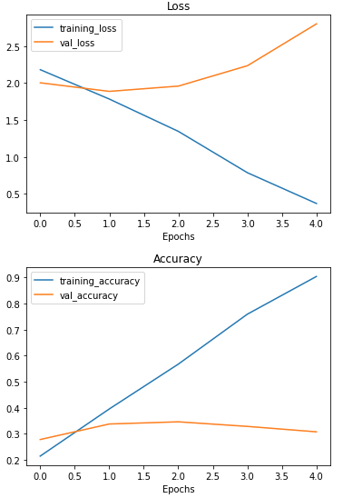
Even with a simplified model, it looks like our model is still dramatically overfitting the training data. What else could we try?
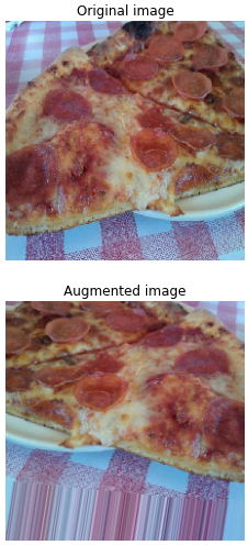
Why don't we try data augmentation?
Data augmentation makes it harder for the model to learn on the training data and in turn, hopefully, makes the patterns it learns more generalizable to unseen data.
To create augmented data, we'll recreate a new ImageDataGenerator instance, this time adding some parameters such as rotation_range and horizontal_flip to manipulate our images.
Let's create an augmented data generation instance
# Create augmented data generator instance
train_datagen_augmented = ImageDataGenerator(rescale=1/255.,
rotation_range=20, # note: this is an int not a float
width_shift_range=0.2,
height_shift_range=0.2,
zoom_range=0.2,
horizontal_flip=True)
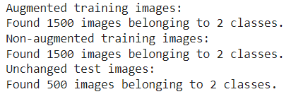
train_data_augmented = train_datagen_augmented.flow_from_directory(train_dir,
target_size=(224, 224),
batch_size=32,
class_mode='categorical')
Rather than rewrite the model from scratch, we can clone it using a handy function in TensorFlow called clone_model which can take an existing model and rebuild it in the same format.
The cloned version will not include any of the weights (patterns) the original model has learned. So when we train it, it'll be like training a model from scratch.
# Clone the model (use the same architecture)
model_f = tf.keras.models.clone_model(model_improve)
# Compile the cloned model (same setup as used for model_improve)
model_f.compile(loss="categorical_crossentropy",
optimizer=tf.keras.optimizers.Adam(),
metrics=["accuracy"])
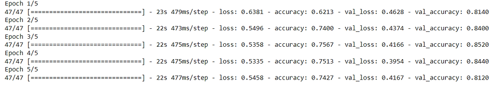
# Fit the model
history_f = model_f.fit(train_data_augmented, # use augmented data
epochs=5,
steps_per_epoch=len(train_data_augmented),
validation_data=test_data,
validation_steps=len(test_data))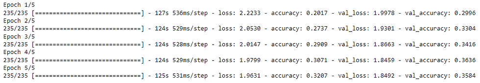
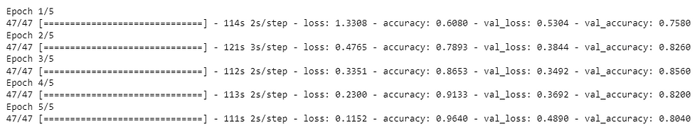
You can see it each epoch takes longer than the previous model. This is because our data is being augmented on the fly on the CPU as it gets loaded onto the GPU, in turn, increasing the amount of time between each epoch.
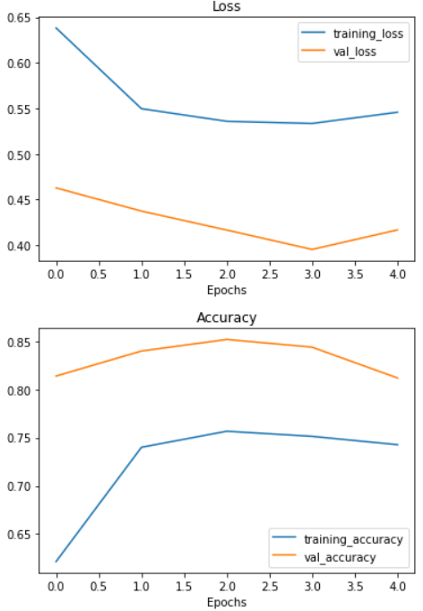
Let's check the performance of augmented data
# Check out our model's performance with augmented data
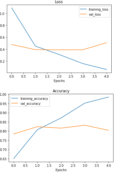
plot_loss_curves(history_f)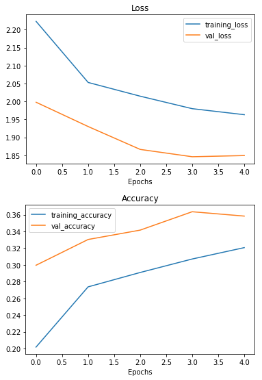
That's looking much better, the loss curves are much closer to each other. Although our model didn't perform as well on the augmented training set, it performed much better on the validation dataset. It even looks like if we kept it training for longer (more epochs) the evaluation metrics might continue to improve.
We would keep trying to improve our model, however, we would make predictions with this model for now,
Making a Prediction
What good is a model if you can't make predictions with it?
Let's first remind ourselves of the classes our multi-class model has been trained on and then we'll download some of our own custom images to work with.
Let's get some custom images
!wget -q https://raw.githubusercontent.com/sumitdeyonline/machinelearning/main/03-hamburgerandfries.jpeg
!wget -q https://raw.githubusercontent.com/sumitdeyonline/machinelearning/main/03-steak.jpeg
!wget -q https://raw.githubusercontent.com/sumitdeyonline/machinelearning/main/03-sushi.jpeg
Okay, we've got some custom images to try, let's use the pred_and_plot function to make a prediction with model_f on one of the images and plot it.
Let's readjust our pred_and_plot function to work with multiple classes as well as binary classes.
# Create a function to import an image and resize it to be able to be used with our model
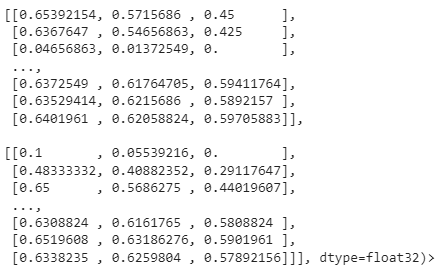
def load_and_prep_image(filename, img_shape=224):
"""
Reads an image from filename, turns it into a tensor
and reshapes it to (img_shape, img_shape, colour_channel).
"""
# Read in target file (an image)
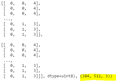
img = tf.io.read_file(filename)
# Decode the read file into a tensor & ensure 3 colour channels
# (our model is trained on images with 3 colour channels and sometimes images have 4 colour channels)
img = tf.image.decode_image(img, channels=3)
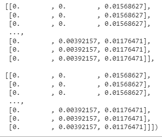
# Resize the image (to the same size our model was trained on)
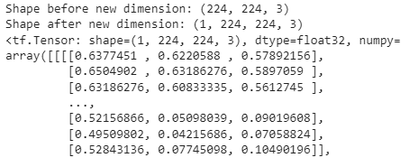
img = tf.image.resize(img, size = [img_shape, img_shape])
# Rescale the image (get all values between 0 and 1)
img = img/255.
return img# Adjust function to work with multi-class
def pred_and_plot(model, filename, class_names):
"""
Imports an image located at filename, makes a prediction on it with
a trained model and plots the image with the predicted class as the title.
"""
# Import the target image and preprocess it
img = load_and_prep_image(filename)
# Make a prediction
pred = model.predict(tf.expand_dims(img, axis=0))
# Get the predicted class
if len(pred[0]) > 1: # check for multi-class
pred_class = class_names[pred.argmax()] # if more than one output, take the max
else:
pred_class = class_names[int(tf.round(pred)[0][0])] # if only one output, round
# Plot the image and predicted class
plt.imshow(img)
plt.title(f"Prediction: {pred_class}")
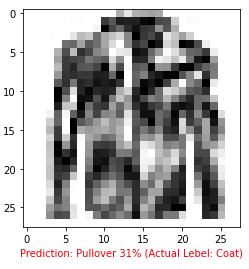
plt.axis(False);Let's try out the prediction
pred_and_plot(model_f, "03-hamburgerandfries.jpeg", class_names)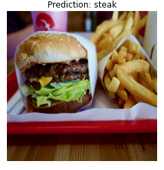
pred_and_plot(model_f, "03-sushi.jpeg", class_names)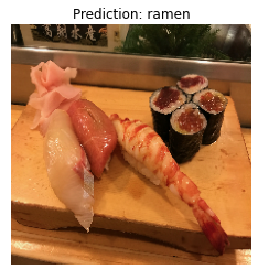
Our model's predictions aren't very good, this is because it's only performing at ~35% accuracy on the test dataset. We can able to do more experiments to improve this model to be more accurate.
In next session we would discuss more about the powerful transfer learning, transfer learning is taking the patterns (also called weights), another model has learned from another problem and using them for our own problem.