Neural Network Regression Problem with TensorFlow(Part 2)
- Sumit Dey
- Feb 23, 2022
- 5 min read
Continue after Part 1
Create a little bit of a bigger dataset and a new model
we'll create a little bit of a bigger dataset(using NumPy) and create new models to compares the predictions.
Let's create the bigger Input Dataset
import tensorflow as tf
import numpy as np
# Make a bigger dataset
X = np.arange(-100, 100, 4)
X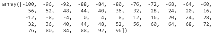
Bigger Output Dataset
# Make labels for the dataset (adhering to the same pattern as before)
y = np.arange(-90, 110, 4)
y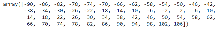
If we add y=X+10, we can make the labels like so:
# Same result as above
y = X + 10
y
Split Dataset into training/test dataset
One of the other most common and important steps in a machine learning project is creating a training and test set (and when required, a validation set) and each set is required for a different purpose
Training set - the model learns from this data, which is typically 70-80% of the total data available (like the course materials you study during the semester).
Validation set - the model gets tuned on this data, which is typically 10-15% of the total data available (like the practice exam you take before the final exam).
Test set - the model gets evaluated on this data to test what it has learned, it's typically 10-15% of the total data available (like the final exam you take at the end of the semester).
Now we need to create Training and Validation dataset by splitting X and y arrays.
# Check how many samples we have
len(X), len(y)
# Split data into train and test sets
X_train = X[:40] # first 40 examples (80% of data)
y_train = y[:40]
X_test = X[40:] # last 10 examples (20% of data)
y_test = y[40:]

len(X_train), len(X_test)
Visualizing the data
Now we have to visualize our data, let's plot a nice colorful plot to visualize the data. using matpotlib.pyplot library to generate a plot
import matplotlib.pyplot as plt
plt.figure(figsize=(10, 7))
# Plot training data in blue
plt.scatter(X_train, y_train, c='b', label='Training data')
# Plot test data in green
plt.scatter(X_test, y_test, c='g', label='Testing data')
# Show the legend
plt.legend();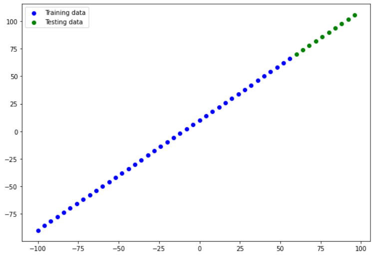
Anytime we can visualize data, model, prediction etc. are a good idea.
Time to build model
With this graph in mind, what we'll be trying to do is build a model which learns the pattern in the blue dots (X_train) to draw the green dots (X_test).
# Set random seed
tf.random.set_seed(42)

# Create a model
model = tf.keras.Sequential([
   tf.keras.layers.Dense(1, input_shape=[1])
   # define the input_shape to our model
])

# Compile model (same as above)
model.compile(loss=tf.keras.losses.mae,
              optimizer=tf.keras.optimizers.SGD(),
              metrics=["mae"])
# Fit the model to the training data
model.fit(X_train, y_train, epochs=100, verbose=0)
# verbose controls how much gets output
Visualizing the predictions
Now we have the trained model, visualize some predictions. To visualize predictions, it's always a good idea to plot them against the ground truth labels.
Often you'll see this in the form of y_test vs. y_pred (ground truth vs. predictions).
First, we'll make some predictions on the test data (X_test), remember the model has never seen the test data.
# Make predictions
y_preds = model.predict(X_test)
# View the predictions
y_preds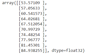
Let's create a plotting function to visualize the data
def plot_predictions(train_data=X_train,
                     train_labels=y_train,
                     test_data=X_test,
                     test_labels=y_test,
                     predictions=y_preds):
"""
Plots training data, test data and compares predictions.
"""
plt.figure(figsize=(10, 7))
# Plot training data in blue
plt.scatter(train_data, train_labels, c="b", label="Training data")
# Plot test data in green
plt.scatter(test_data, test_labels, c="g", label="Testing data")
# Plot the predictions in red (predictions were made on the test data)
plt.scatter(test_data, predictions, c="r", label="Predictions")
# Show the legend
plt.legend();
Now we are getting plot using this function
plot_predictions(train_data=X_train,
                 train_labels=y_train,
                 test_data=X_test,
                 test_labels=y_test,
                 predictions=y_preds)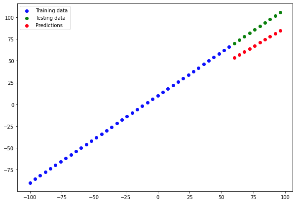
We can see, our predictions aren't totally correct, we can do more experiments to improve this result.
Running experiments to improve a model
There are many ways to improve your model, please find the most common way to do it
Get more data - get more examples for your model to train on (more opportunities to learn patterns).
Make your model larger (use a more complex model) - this might come in the form of more layers or more hidden units in each layer.
Train for longer - give your model more of a chance to find the patterns in the data.
In a real-world situation, we would not be able to change data, let's experiment with the 2 and 3. Let's create three models with the following scenarios
model_1 - same as the original model, trained for 100 epochs.
model_2 - 2 layers, trained for 100 epochs.
model_3 - 2 layers, trained for 500 epochs.
Build model_1
# Set random seed
tf.random.set_seed(42)

# Replicate original model
model_1 = tf.keras.Sequential([
  tf.keras.layers.Dense(1)
])

# Compile model
model_1.compile(loss=tf.keras.losses.mae,
              optimizer=tf.keras.optimizers.SGD(),
              metrics=["mae"])

# Fit the model to the training data
model_1.fit(tf.expand_dims(X_train, axis=-1), y_train, epochs=100)
-----
-----
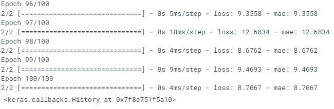
Let's make predictions for model_1
# Make and plot predictions for model_1
y_preds_1 = model_1.predict(X_test)
plot_predictions(predictions=y_preds_1)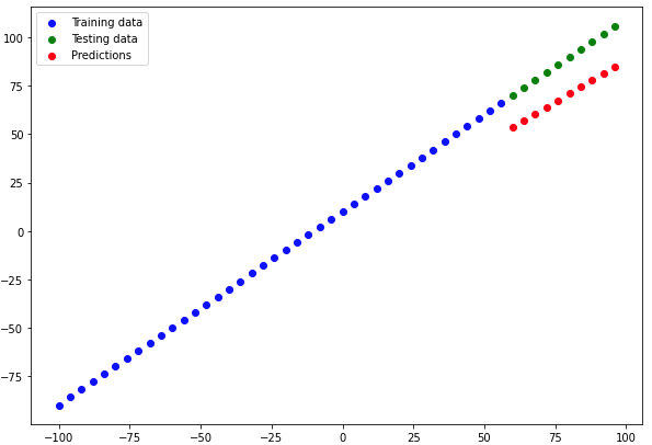
Not much improvement from the previous model, let's build model_2
Build model_2
This time we are adding an extra dense layer, keeping everything else the same
# Set random seed
tf.random.set_seed(42)

# Replicate model_1 and add an extra layer
model_2 = tf.keras.Sequential([
  tf.keras.layers.Dense(1),
  tf.keras.layers.Dense(1) # add a second layer,
])
# Compile model
model_2.compile(loss=tf.keras.losses.mae,
              optimizer=tf.keras.optimizers.SGD(),
              metrics=["mae"])

# Fit the model to the training data
model_2.fit(tf.expand_dims(X_train, axis=-1), y_train, epochs=100, verbose=0) # set verbose to 0 for less output 
Let's predict for the model_2
# Make and plot predictions for model_2
y_preds_2 = model_2.predict(X_test)
plot_predictions(predictions=y_preds_2)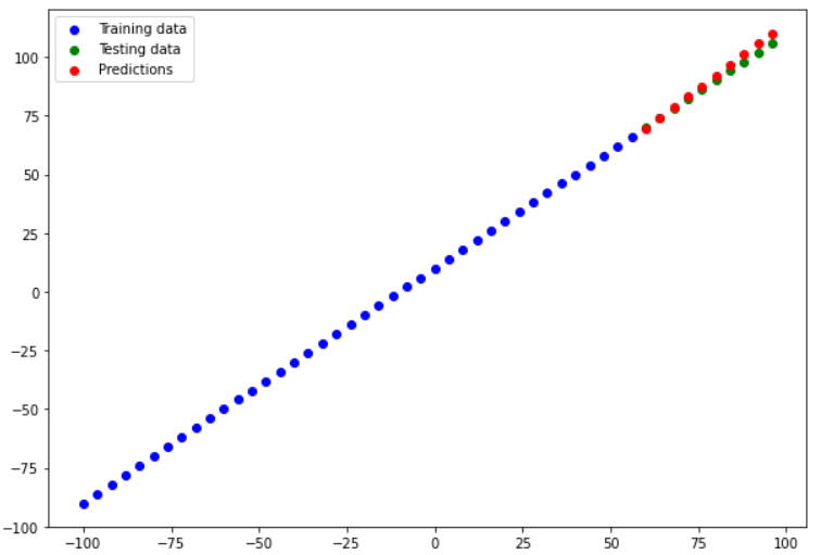
It's looking far better than model_1 after adding an extra layer, let's try to build the third model, everything keeps the same as model_2 except train for longer(500 instead of 100)
Build model_3
Train this model for 500 epochs
# Set random seed
tf.random.set_seed(42)

# Replicate model_2
model_3 = tf.keras.Sequential([
  tf.keras.layers.Dense(1),
  tf.keras.layers.Dense(1) # add a second layer,
])
# Compile model
model_3.compile(loss=tf.keras.losses.mae,
              optimizer=tf.keras.optimizers.SGD(),
              metrics=["mae"])

# Fit the model to the training data
model_3.fit(tf.expand_dims(X_train, axis=-1), y_train, epochs=500, verbose=0) # set verbose to 0 for less output
Let's predict the model_3
# Make and plot predictions for model_3
y_preds_3 = model_3.predict(X_test)
plot_predictions(predictions=y_preds_3)
It is really strange, model performance has been worse when trained for longer. As it turns out that when you train a model too long, the result can be worse.
Comparing the results
Now we got results of three similar models, we need to compare the results.
Before we compare the three models, create two functions to get the mean absolute error and mean squared error value for test data and predictions.
def mae(y_test, y_pred):
  """  Calculuates mean absolute error between y_test and y_preds.
  """
  return tf.metrics.mean_absolute_error(y_test,
                                        y_pred)

 def mse(y_test, y_pred):
   """
   Calculates mean squared error between y_test and y_preds.
   """
   return tf.metrics.mean_squared_error(y_test,
                                        y_pred)
Now we are calculating mae and mse for all three models
# Calculate model_1 metrics
mae_1 = mae(y_test, y_preds_1.squeeze()).numpy()
mse_1 = mse(y_test, y_preds_1.squeeze()).numpy()
mae_1, mse_1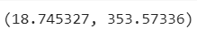
# Calculate model_2 metrics
mae_2 = mae(y_test, y_preds_2.squeeze()).numpy()
mse_2 = mse(y_test, y_preds_2.squeeze()).numpy()
mae_2, mse_2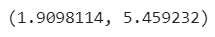
# Calculate model_3 metrics
mae_3 = mae(y_test, y_preds_3.squeeze()).numpy()
mse_3 = mse(y_test, y_preds_3.squeeze()).numpy()
mae_3, mse_3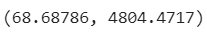
Let's compare the model
import pandas as pd
model_results = [["model_1", mae_1, mse_1],
                 ["model_2", mae_2, mse_2],
                 ["model_3", mae_3, mae_3]]
all_results = pd.DataFrame(model_results, columns=["model", "mae", "mse"])
all_results 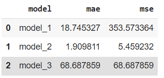
The results of our experiment are that model_2 performance is the best out of the three models. Comparing models is tedious, in this case, we are comparing three models, in the real-world scenario we may need to compare more models.
But this is part of what machine learning modeling is about, trying many different combinations of models and seeing which performs best.
Another thing you'll also find is what you thought may work (such as training a model for longer) may not always work and the exact opposite is also often the case.


Comments