- Sumit Dey
- Mar 19, 2022
- 15 min read
This blog is the continuation of Transfer Learning Part 1
In the previous blogs, we observed transfer learning is getting far better results on the Food Vision experiment than our own models, even with the less dataset.
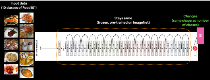
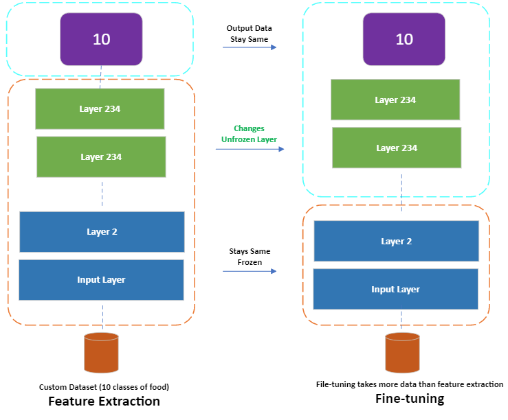
In this blog, we would discuss the fine-tuning transfer learning, pre-trained model are unfrozen and tweaked to better suit our data. For feature extraction transfer learning, you may only train the top 1-3 layers of a pre-trained model with your own data, in fine-tuning transfer learning, you might train 1-3+ layers of a pre-trained model (where the '+' indicates that many or all of the layers could be trained).
First, let's create a few functions to help with the repetitive tasks below, rewriting the same code becomes tedious.
import tensorflow as tf
import datetime
import matplotlib.pyplot as plt
import zipfile
import os

def create_tensorboard_callback(dir_name, experiment_name):
  """
  Creates a TensorBoard callback instand to store log files.

  Stores log files with the filepath:
    "dir_name/experiment_name/current_datetime/"

  Args:
    dir_name: target directory to store TensorBoard log files
    experiment_name: name of experiment directory (e.g. efficientnet_model_1)
  """
  log_dir = dir_name + "/" + experiment_name + "/" + datetime.datetime.now().strftime("%Y%m%d-%H%M%S")
  tensorboard_callback = tf.keras.callbacks.TensorBoard(
      log_dir=log_dir
  )
  print(f"Saving TensorBoard log files to: {log_dir}")
  return tensorboard_callback


# Plot the validation and training data separately
def plot_loss_curves(history):
  """
  Returns separate loss curves for training and validation metrics.

  Args:
    history: TensorFlow model History object (see: https://www.tensorflow.org/api_docs/python/tf/keras/callbacks/History)
  """
  loss = history.history['loss']
  val_loss = history.history['val_loss']

  accuracy = history.history['accuracy']
  val_accuracy = history.history['val_accuracy']

  epochs = range(len(history.history['loss']))

  # Plot loss
  plt.plot(epochs, loss, label='training_loss')
  plt.plot(epochs, val_loss, label='val_loss')
  plt.title('Loss')
  plt.xlabel('Epochs')
  plt.legend()

  # Plot accuracy
  plt.figure()
  plt.plot(epochs, accuracy, label='training_accuracy')
  plt.plot(epochs, val_accuracy, label='val_accuracy')
  plt.title('Accuracy')
  plt.xlabel('Epochs')
  plt.legend();

# Create function to unzip a zipfile into current working directory
# (since we're going to be downloading and unzipping a few files)

def unzip_data(filename):
  """
  Unzips filename into the current working directory.

  Args:
    filename (str): a filepath to a target zip folder to be unzipped.
  """
  zip_ref = zipfile.ZipFile(filename, "r")
  zip_ref.extractall()
  zip_ref.close()

# Walk through an image classification directory and find out how many files (images)
# are in each subdirectory.

def walk_through_dir(dir_path):
  """
  Walks through dir_path returning its contents.

  Args:
    dir_path (str): target directory

  Returns:
    A print out of:
      number of subdiretories in dir_path
      number of images (files) in each subdirectory
      name of each subdirectory
  """
  for dirpath, dirnames, filenames in os.walk(dir_path):
    print(f"There are {len(dirnames)} directories and {len(filenames)} images in '{dirpath}'.")
Working with less Data(Food Classes)
In my previous blog, we see we could get great results using 10% training data using transfer learning. in this blog, we're going to continue to work with smaller subsets of the data, except this time we'll have a look at how we can use the in-built pre-trained models within the tf.keras.applications module as well as how to fine-tune them to our own custom dataset. Finally, we'll also be practicing using the Keras Functional API for building deep learning models. The Functional API is a more flexible way to create models than the tf.keras.Sequential API.
Let's start downloading some data
# Get 10% of the data of the 10 classes
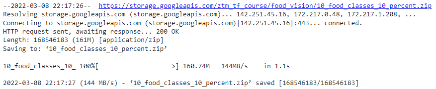
!wget https://storage.googleapis.com/ztm_tf_course/food_vision/10_food_classes_10_percent.zip
unzip_data("10_food_classes_10_percent.zip")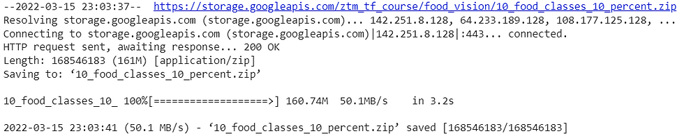
The dataset we're downloading is the 10 food classes dataset (from Food 101) with 10% of the training images we used in the previous blog.
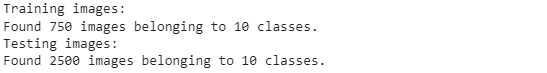
# Walk through 10 percent data directory and list number of files
walk_through_dir("10_food_classes_10_percent")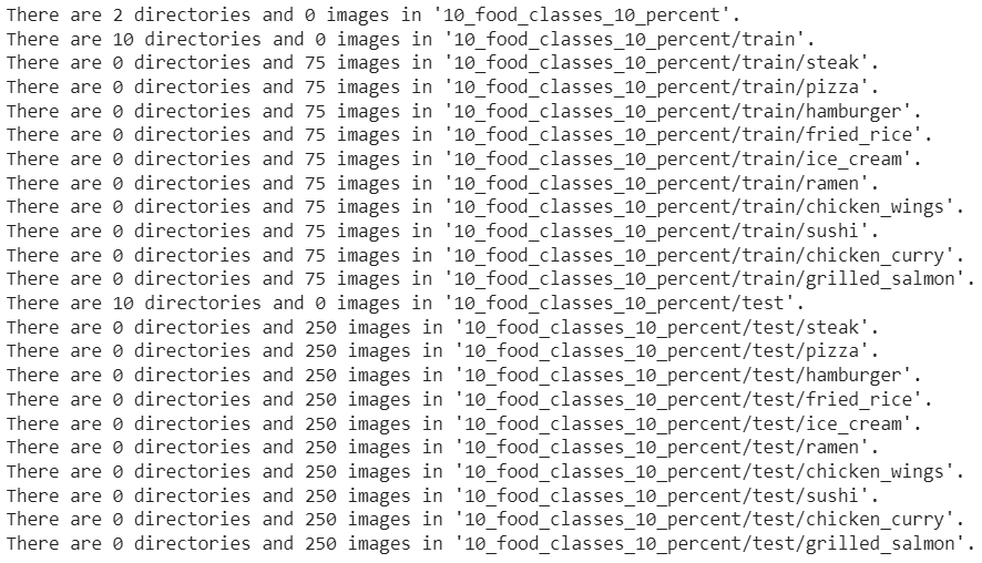
We can see that each of the training directories contains 75 images and each of the testing directories contain 250 images.
Let's define our training and test file paths.
# Create training and test directories
train_dir = "10_food_classes_10_percent/train/"
test_dir = "10_food_classes_10_percent/test/"
Now we've got some image data, we need a way of loading it into a TensorFlow compatible format. Previously, we've used the ImageDataGenerator class. And while this works well and is still very commonly used, this time we're going to use the image_data_from_directory function.
One of the main benefits of using tf.keras.prepreprocessing.image_dataset_from_directory() rather than ImageDataGenerator is that it creates a tf.data.Dataset object rather than a generator. The main advantage of this is the tf.data.Dataset API is much more efficient (faster) than the ImageDataGenerator API which is paramount for larger datasets.
Let's see how it looks
# Create data inputs
import tensorflow as tf
IMG_SIZE = (224, 224) # define image size
train_data_10_percent = tf.keras.preprocessing.image_dataset_from_directory(directory=train_dir,
                                                    image_size=IMG_SIZE,
                                               label_mode="categorical",
                                             # what type are the labels?
                                                    batch_size=32)
            # batch_size is 32 by default, this is generally a good number
test_data_10_percent = tf.keras.preprocessing.image_dataset_from_directory(directory=test_dir,
                                                    image_size=IMG_SIZE,
                                                label_mode="categorical")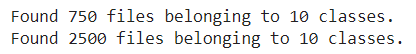
The main parameters we're concerned about in the image_dataset_from_directory() function are:
directory - the filepath of the target directory we're loading images in from.
image_size - the target size of the images we're going to load in (height, width).
batch_size - the batch size of the images we're going to load in. For example, if the batch_size is 32 (the default), batches of 32 images and labels at a time will be passed to the model.
There are more we could play around with if we needed to in the tf.keras.preprocessing documentation.
Let's check the training dataset type, shape etc.
# Check the training data datatype
train_data_10_percent
In the above output:
(None, 224, 224, 3) refers to the tensor shape of our images where None is the batch size, 224 is the height (and width) and 3 is the color channels (red, green, blue).
(None, 10) refers to the tensor shape of the labels where None is the batch size and 10 is the number of possible labels (the 10 different food classes).
Both image tensors and labels are of the datatype tf.float32.
The batch_size is None due to it only being used during model training. You can think of a placeholder waiting to be filled with the batch_size parameter from image_dataset_from_directory().
Another benefit of using the tf.data.Dataset API is the associated method that comes with it.
For example, if we want to find the name of the classes we were working with, we could use the class_names attribute.
# Check out the class names of our dataset
train_data_10_percent.class_names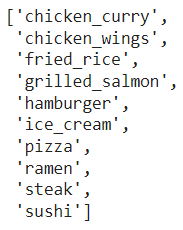
if we wanted to see an example batch of data, we could use the take() method.
# See an example batch of data
for images, labels in train_data_10_percent.take(1):
  print(images, labels)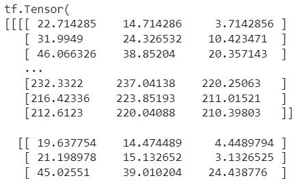
------
------
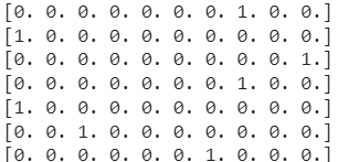
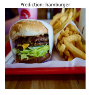
Notice how the image arrays come out as tensors of pixel values where as the labels come out as one-hot encodings (e.g. [0. 0. 0. 0. 1. 0. 0. 0. 0. 0.] for hamburger).
Building a transfer learning model using the Keras Functional API
To do so we're going to be using the tf.keras.applications module as it contains a series of already trained (on ImageNet) computer vision models as well as the Keras Functional API to construct our model.
We're going to go through the following steps:
Instantiate a pre-trained base model object by choosing a target model such as EfficientNetB0 from tf.keras.applications, setting the include_top parameter to False (we do this because we're going to create our own top, which are the output layers for the model).
Set the base model's trainable attribute to False to freeze all of the weights in the pre-trained model.
Define an input layer for our model, for example, what shape of data should our model expect?
[Optional] Normalize the inputs to our model if requires. Some computer vision models such as ResNetV250 require their inputs to be between 0 & 1.
Pass the inputs to the base model.
Pool the outputs of the base model into a shape compatible with the output activation layer (turn base model output tensors into same shape as label tensors). This can be done using tf.keras.layers.GlobalAveragePooling2D() or tf.keras.layers.GlobalMaxPooling2D() though the former is more common in practice.
Create an output activation layer using tf.keras.layers.Dense() with the appropriate activation function and number of neurons.
Combine the inputs and outputs layer into a model using tf.keras.Model().
Compile the model using the appropriate loss function and choose of optimizer.
Fit the model for desired number of epochs and with necessary callbacks (in our case, we'll start off with the TensorBoard callback).
Let's create the base model
# 1. Create base model with tf.keras.applications
base_model = tf.keras.applications.EfficientNetB0(include_top=False)
# 2. Freeze the base model (so the pre-learned patterns remain)
base_model.trainable = False
# 3. Create inputs into the base model
inputs = tf.keras.layers.Input(shape=(224, 224, 3), name="input_layer")
# 4. If using ResNet50V2, add this to speed up convergence, remove for EfficientNet
# x = tf.keras.layers.experimental.preprocessing.Rescaling(1./255)(inputs)
# 5. Pass the inputs to the base_model (note: using tf.keras.applications, EfficientNet inputs don't have to be normalized)
x = base_model(inputs)
# Check data shape after passing it to base_model
print(f"Shape after base_model: {x.shape}")
# 6. Average pool the outputs of the base model (aggregate all the most important information, reduce number of computations)
x = tf.keras.layers.GlobalAveragePooling2D(name="global_average_pooling_layer")(x)
print(f"After GlobalAveragePooling2D(): {x.shape}")
# 7. Create the output activation layer
outputs = tf.keras.layers.Dense(10, activation="softmax", name="output_layer")(x)
# 8. Combine the inputs with the outputs into a model
model_0 = tf.keras.Model(inputs, outputs)
# 9. Compile the model
model_0.compile(loss='categorical_crossentropy',
optimizer=tf.keras.optimizers.Adam(),
metrics=["accuracy"])
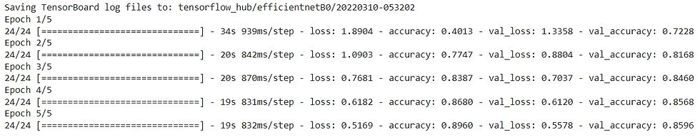
# 10. Fit the model (we use less steps for validation so it's faster)
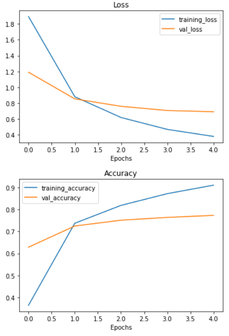
history_10_percent = model_0.fit(train_data_10_percent,
epochs=5,
steps_per_epoch=len(train_data_10_percent),
validation_data=test_data_10_percent,
# Go through less of the validation data so epochs are faster (we want faster experiments!)
validation_steps=int(0.25 * len(test_data_10_percent)),
# Track our model's training logs for visualization later
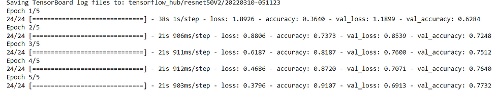
callbacks=[create_tensorboard_callback("transfer_learning", "10_percent_feature_extract")])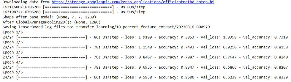
It seems training our model performs incredibly well on both the training (87%+ accuracy) and test sets (~83% accuracy). Now we need to inspect the model, start with base model.
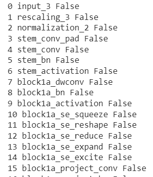
# Check layers in our base model
for layer_number, layer in enumerate(base_model.layers):
  print(layer_number, layer.name)
--------
--------
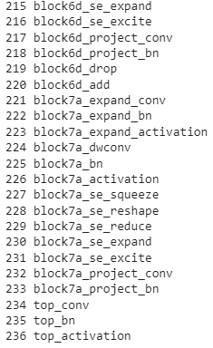
That's a lot of layers... to hand code all of those would've taken a fairly long time to do, yet we can still take advantage of them thanks to the power of transfer learning.
Let's find the summary of the base model
base_model.summary()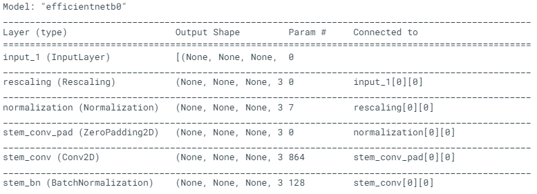
--------
--------
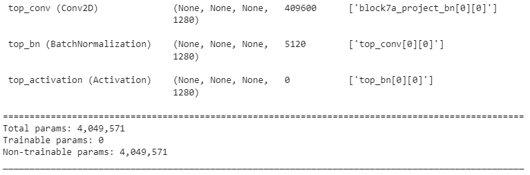
You can see how each of the different layers has a certain number of parameters. Since we are using a pre-trained model, you can think of all of these parameters are patterns the base model has learned on another dataset. And because we set base_model.trainable = False, these patterns remain as they are during training (they're frozen and don't get updated).
Let's see the summary of our overall model.
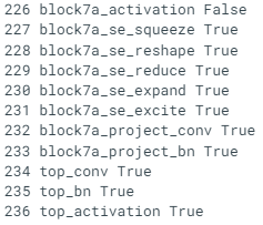
# Check summary of model constructed with Functional API
model_0.summary()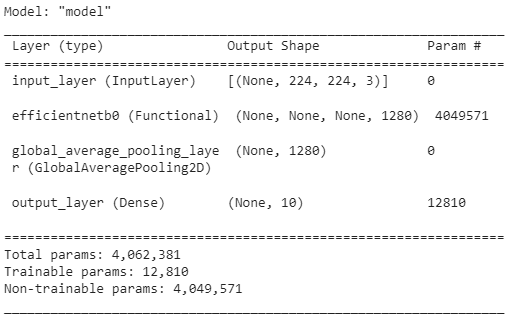
Our overall model has five layers but really, one of those layers (efficientnetb0) has 236 layers. You can see how the output shape started out as (None, 224, 224, 3) for the input layer (the shape of our images) but was transformed to be (None, 10) by the output layer (the shape of our labels), where None is the placeholder for the batch size.
Getting a feature vector from a trained model
The tf.keras.layers.GlobalAveragePooling2D() layer transforms a 4D tensor into a 2D tensor by averaging the values across the inner-axes. Let's see an example
# Define input tensor shape (same number of dimensions as the output of efficientnetb0)
input_shape = (1, 4, 4, 3)

# Create a random tensor
tf.random.set_seed(42)
input_tensor = tf.random.normal(input_shape)
print(f"Random input tensor:\n {input_tensor}\n")

# Pass the random tensor through a global average pooling 2D layer
global_average_pooled_tensor = tf.keras.layers.GlobalAveragePooling2D()(input_tensor)
print(f"2D global average pooled random tensor:\n {global_average_pooled_tensor}\n")

# Check the shapes of the different tensors
print(f"Shape of input tensor: {input_tensor.shape}")
print(f"Shape of 2D global averaged pooled input tensor: {global_average_pooled_tensor.shape}")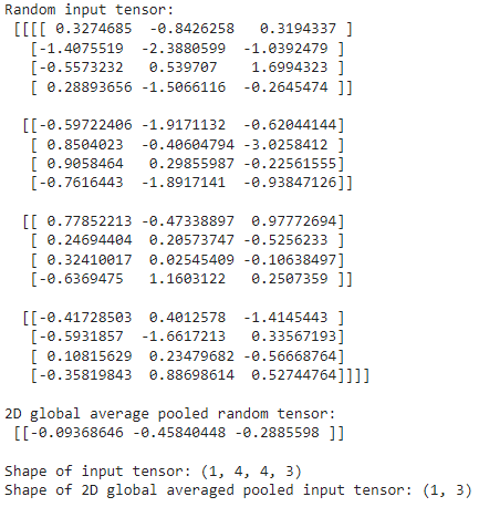
You can see the tf.keras.layers.GlobalAveragePooling2D() layer condensed the input tensor from shape (1, 4, 4, 3) to (1, 3). It did so by averaging the input_tensor across the middle two axes.
Running a series of transfer learning experiments
We've seen the incredible results of transfer learning on 10% of the training data, what about 1% of the training data?
Why don't we answer that question while running the following modeling experiments:
Use feature extraction transfer learning on 1% of the training data with data augmentation.
Use feature extraction transfer learning on 10% of the training data with data augmentation.
Use fine-tuning transfer learning on 10% of the training data with data augmentation.
Use fine-tuning transfer learning on 100% of the training data with data augmentation.
While all of the experiments will be run on different versions of the training data, they will all be evaluated on the same test dataset, this ensures the results of each experiment are as comparable as possible.
All experiments will be done using the EfficientNetB0 model within the tf.keras.applications module.
Let's begin by downloading the data for experiment 1, using feature extraction transfer learning on 1% of the training data with data augmentation.
# Download and unzip data
!wget https://storage.googleapis.com/ztm_tf_course/food_vision/10_food_classes_1_percent.zip
unzip_data("10_food_classes_1_percent.zip")

# Create training and test dirs
train_dir_1_percent = "10_food_classes_1_percent/train/"
test_dir = "10_food_classes_1_percent/test/"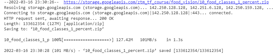
How many images are we working with?
# Walk through 1 percent data directory and list number of files
walk_through_dir("10_food_classes_1_percent")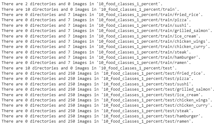
Time to load our images in as tf.data.Dataset objects, to do so, we'll use the image_dataset_from_directory() method.
import tensorflow as tf
IMG_SIZE = (224, 224)
train_data_1_percent = tf.keras.preprocessing.image_dataset_from_directory(train_dir_1_percent,
                                               label_mode="categorical",
                                               batch_size=32, # default
                                                                           image_size=IMG_SIZE)
test_data = tf.keras.preprocessing.image_dataset_from_directory(test_dir,
                                                 label_mode="categorical",
                                                 image_size=IMG_SIZE)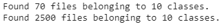
Adding data augmentation right into the model
Data loaded, time to augment it. Using the tf.keras.layers.experimental.preprocessing module and creating a dedicated data augmentation layer.
The data augmentation transformations we're going to use are:
RandomFlip - flips image on the horizontal or vertical axis.
RandomRotation - randomly rotates the image by a specified amount.
RandomZoom - randomly zooms into an image by a specified amount.
RandomHeight - randomly shifts image height by a specified amount.
RandomWidth - randomly shifts image width by a specified amount.
Rescaling - normalizes the image pixel values to be between 0 and 1, this is worth mentioning because it is required for some image models but since we're using the tf.keras.applications implementation of EfficientNetB0, it's not required.
Feature extraction transfer learning on 1% of the data with data augmentation
from tensorflow.keras import layers
from tensorflow.keras.layers.experimental import preprocessing

# Setup input shape and base model, freezing the base model layers
input_shape = (224, 224, 3)
base_model = tf.keras.applications.EfficientNetB0(include_top=False)
base_model.trainable = False

# Create input layer
inputs = layers.Input(shape=input_shape, name="input_layer")

# Add in data augmentation Sequential model as a layer
x = data_augmentation(inputs)

# Give base_model inputs (after augmentation) and don't train it
x = base_model(x, training=False)

# Pool output features of base model
x = layers.GlobalAveragePooling2D(name="global_average_pooling_layer")(x)

# Put a dense layer on as the output
outputs = layers.Dense(10, activation="softmax", name="output_layer")(x)

# Make a model with inputs and outputs
model_1 = keras.Model(inputs, outputs)

# Compile the model
model_1.compile(loss="categorical_crossentropy",
              optimizer=tf.keras.optimizers.Adam(),
              metrics=["accuracy"])

# Fit the model
history_1_percent = model_1.fit(train_data_1_percent,
                    epochs=5,
                    steps_per_epoch=len(train_data_1_percent),
                    validation_data=test_data,
                    validation_steps=int(0.25* len(test_data)), # validate for less steps
                    # Track model training logs
                    callbacks=[create_tensorboard_callback("transfer_learning", "1_percent_data_aug")])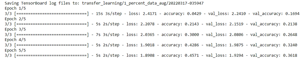
Using only 7 training images per class, using transfer learning our model was able to get ~40% accuracy on the validation set. This result is pretty amazing since the original Food-101 paper achieved 50.67% accuracy with all the data, namely, 750 training images per class.
The important thing to remember is data augmentation only runs during training. So if we were to evaluate or use our model for inference (predicting the class of an image) the data augmentation layers will be automatically turned off.
# Evaluate on the test data
results_1_percent_data_aug = model_1.evaluate(test_data)
results_1_percent_data_aug
The results here may be slightly better/worse than the log outputs of our model during training because during training we only evaluate our model on 25% of the test data using the line validation_steps=int(0.25 * len(test_data)). Doing this speeds up our epochs but still gives us enough of an idea of how our model is going.
After many experiments we would try the 5th experiment, that is fine-tuning an existing model all of the data
Fine-tuning an existing model all of the data
Let's try all data from 10 food classes
# Download and unzip 10 classes of data with all images
!wget https://storage.googleapis.com/ztm_tf_course/food_vision/10_food_classes_all_data.zip
unzip_data("10_food_classes_all_data.zip")

# Setup data directories
train_dir = "10_food_classes_all_data/train/"
test_dir = "10_food_classes_all_data/test/"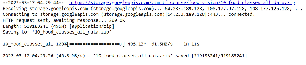
# How many images are we working with now?
walk_through_dir("10_food_classes_all_data")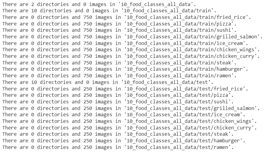
And now we'll turn the images into tensors datasets.
# Setup data inputs
import tensorflow as tf
IMG_SIZE = (224, 224)
train_data_10_classes_full = tf.keras.preprocessing.image_dataset_from_directory(train_dir,
                                                                                 label_mode="categorical",
                                                                                 image_size=IMG_SIZE)

# Note: this is the same test dataset we've been using for the previous modelling experiments
test_data = tf.keras.preprocessing.image_dataset_from_directory(test_dir,
                                                                label_mode="categorical",
                                                                image_size=IMG_SIZE)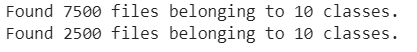
Oh, this is looking good. We've got 10x more images in of the training classes to work with.
The test dataset is the same we've been using for our previous experiments.
As it is now, our model_2 has been fine-tuned on 10 percent of the data, so to begin fine-tuning on all of the data and keep our experiments consistent, we need to revert it back to the weights we checkpointed after 5 epochs of feature-extraction.
Let's create a model
# Create a functional model with data augmentation
import tensorflow as tf
from tensorflow.keras import layers
from tensorflow.keras.layers.experimental import preprocessing
from tensorflow.keras.models import Sequential

# Build data augmentation layer
data_augmentation = Sequential([
  preprocessing.RandomFlip('horizontal'),
  preprocessing.RandomHeight(0.2),
  preprocessing.RandomWidth(0.2),
  preprocessing.RandomZoom(0.2),
  preprocessing.RandomRotation(0.2),
  # preprocessing.Rescaling(1./255) # keep for ResNet50V2, remove for EfficientNet
], name="data_augmentation")

# Setup the input shape to our model
input_shape = (224, 224, 3)

# Create a frozen base model
base_model = tf.keras.applications.EfficientNetB0(include_top=False)
base_model.trainable = False

# Create input and output layers
inputs = layers.Input(shape=input_shape, name="input_layer") # create input layer
x = data_augmentation(inputs) # augment our training images
x = base_model(x, training=False) # pass augmented images to base model but keep it in inference mode, so batchnorm layers don't get updated: https://keras.io/guides/transfer_learning/#build-a-model
x = layers.GlobalAveragePooling2D(name="global_average_pooling_layer")(x)
outputs = layers.Dense(10, activation="softmax", name="output_layer")(x)
model_2 = tf.keras.Model(inputs, outputs)

# Compile
model_2.compile(loss="categorical_crossentropy",
              optimizer=tf.keras.optimizers.Adam(lr=0.001), # use Adam optimizer with base learning rate
              metrics=["accuracy"])
Creating a ModelCheckpoint callback
Our model is compiled and ready to be fit, so why haven't we fit it yet?
Well, for this experiment we're going to introduce a new callback, the ModelCheckpoint callback. The ModelCheckpoint callback gives you the ability to save your model, as a whole in the SavedModel for mat or the weights (patterns) only to a specified directory as it trains. This is helpful if you think your model is going to be training for a long time and you want to make backups of it as it trains. It also means if you think your model could benefit from being trained for longer, you can reload it from a specific checkpoint and continue training from there.
For example, say you fit a feature extraction transfer learning model for 5 epochs and you check the training curves and see it was still improving and you want to see if fine-tuning for another 5 epochs could help, you can load the checkpoint, unfreeze some (or all) of the base model layers and then continue training.
But first, let's create a ModelCheckpoint callback. To do so, we have to specify a directory we'd like to save to.
# Setup checkpoint path
checkpoint_path = "ten_percent_model_checkpoints_weights/checkpoint.ckpt" # note: remember saving directly to Colab is temporary

# Create a ModelCheckpoint callback that saves the model's weights only
checkpoint_callback = tf.keras.callbacks.ModelCheckpoint(filepath=checkpoint_path,
                                                         save_weights_only=True, # set to False to save the entire model
                                                         save_best_only=False, # set to True to save only the best model instead of a model every epoch
                                                         save_freq="epoch", # save every epoch
                                                         verbose=1)
The SavedModel format saves a model's architecture, weights, and training configuration all in one folder. It makes it very easy to reload your model exactly how it is elsewhere. However, if you do not want to share all of these details with others, you may want to save and share the weights only (these will just be large tensors of non-human interpretable numbers). If disk space is an issue, saving the weights only is faster and takes up less space than saving the whole model.
Time to fit the model. Because we're going to be fine-tuning it later, we'll create a variable initial_epochs and set it to 5 to use later.
history_10_percent_data_aug = model_2.fit(train_data_10_percent,
                                          epochs=initial_epochs,
                                          validation_data=test_data,
                                          validation_steps=int(0.25 * len(test_data)), # do less steps per validation (quicker)
                                          callbacks=[create_tensorboard_callback("transfer_learning", "10_percent_data_aug"),
                                                     checkpoint_callback])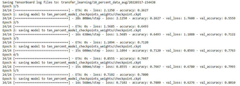
Let's evaluate the model
# Evaluate model (this is the fine-tuned 10 percent of data version)
model_2.evaluate(test_data)
Alright, the previous steps might seem quite confusing but all we've done is:
Trained a feature extraction transfer learning model for 5 epochs on 10% of the data (with all base model layers frozen) and saved the model's weights using ModelCheckpoint.
Fine-tuned the same model on the same 10% of the data for a further 5 epochs with the top 10 layers of the base model unfrozen.
Saved the results and training logs each time.
Reloaded the model from 1 to do the same steps as 2 but with all of the data.
we're going to fine-tune the last 10 layers of the base model with the full dataset for another 5 epochs but first let's remind ourselves which layers are trainable.
# Check which layers are tuneable in the whole model
for layer_number, layer in enumerate(model_2.layers):
  print(layer_number, layer.name, layer.trainable)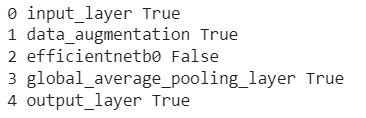
To begin fine-tuning, we'll unfreeze the entire base model by setting its trainable attribute to True. Then we'll refreeze every layer in the base model except for the last 10 by looping through them and setting their trainable attribute to False. Finally, we'll recompile the model.
base_model.trainable = True

# Freeze all layers except for the
for layer in base_model.layers[:-10]:
  layer.trainable = False

# Recompile the model (always recompile after any adjustments to a model)
model_2.compile(loss="categorical_crossentropy",
              optimizer=tf.keras.optimizers.Adam(lr=0.0001), # lr is 10x lower than before for fine-tuning
              metrics=["accuracy"])
Can we get a little more specific?
------
------
It seems all layers except for the last 10 are frozen and untrainable. This means only the last 10 layers of the base model along with the output layer will have their weights updated during training. In our case, we're using the exact same loss, optimizer, and metrics as before, except this time the learning rate for our optimizer will be 10x smaller than before (0.0001 instead of Adam's default of 0.001). We do this so the model doesn't try to overwrite the existing weights in the pre-trained model too fast. In other words, we want learning to be more gradual.
Time to fine-tune!
We're going to continue training from where our previous model finished. Since it trained for 5 epochs, our fine-tuning will begin on epoch 5 and continue for another 5 epochs.
To do this, we can use the initial_epoch parameter of the fit() method. We'll pass it to the last epoch of the previous model's training history (history_10_percent_data_aug.epoch[-1]).
# Fine tune for another 5 epochs

fine_tune_epochs = initial_epochs + 5

# Refit the model (same as model_2 except with more trainable layers)
history_fine_10_percent_data_aug = model_2.fit(train_data_10_percent,
                                               epochs=fine_tune_epochs,
                                               validation_data=test_data,
                                               initial_epoch=history_10_percent_data_aug.epoch[-1], # start from previous last epoch
                                               validation_steps=int(0.25 * len(test_data)),
                                               callbacks=[create_tensorboard_callback("transfer_learning", "10_percent_fine_tune_last_10")]) # name experiment appropriately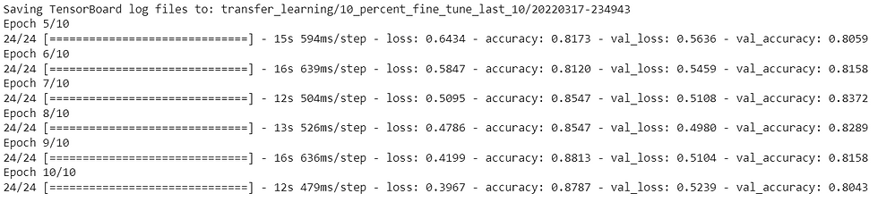
Let's evaluate it.
# Evaluate the model on the test data
results_fine_tune_10_percent = model_2.evaluate(test_data)
Remember, the results from evaluating the model might be slightly different to the outputs from training since during training we only evaluate on 25% of the test data.
Alright, we need a way to evaluate our model's performance before and after fine-tuning. How about we write a function to compare the before and after?
def compare_historys(original_history, new_history, initial_epochs=5):
"""
Compares two model history objects.
"""
# Get original history measurements
acc = original_history.history["accuracy"]
loss = original_history.history["loss"]
print(len(acc))
val_acc = original_history.history["val_accuracy"]
val_loss = original_history.history["val_loss"]
# Combine original history with new history
total_acc = acc + new_history.history["accuracy"]
total_loss = loss + new_history.history["loss"]
total_val_acc = val_acc + new_history.history["val_accuracy"]
total_val_loss = val_loss + new_history.history["val_loss"]
print(len(total_acc))
print(total_acc)
# Make plots
plt.figure(figsize=(8, 8))
plt.subplot(2, 1, 1)
plt.plot(total_acc, label='Training Accuracy')
plt.plot(total_val_acc, label='Validation Accuracy')
plt.plot([initial_epochs-1, initial_epochs-1],
plt.ylim(), label='Start Fine Tuning') # reshift plot around epochs
plt.legend(loc='lower right')
plt.title('Training and Validation Accuracy')
plt.subplot(2, 1, 2)
plt.plot(total_loss, label='Training Loss')
plt.plot(total_val_loss, label='Validation Loss')
plt.plot([initial_epochs-1, initial_epochs-1],
plt.ylim(), label='Start Fine Tuning') # reshift plot around epochs
plt.legend(loc='upper right')
plt.title('Training and Validation Loss')
plt.xlabel('epoch')
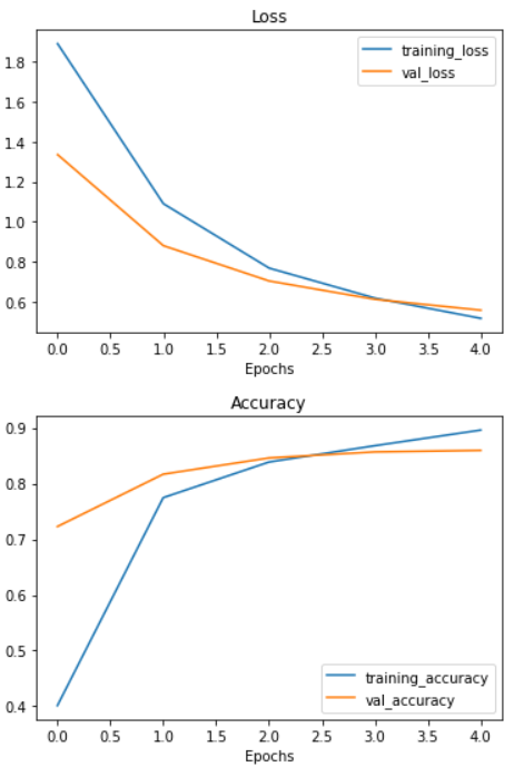
plt.show()This is where saving the history variables of our model training comes in handy. Let's see what happened after fine-tuning the last 10 layers of our model.
compare_historys(original_history=history_10_percent_data_aug,
                 new_history=history_fine_10_percent_data_aug,
                 initial_epochs=5)
Seems like the curves are heading in the right direction after fine-tuning. But remember, it should be noted that fine-tuning usually works best with larger amounts of data.
Fine-tuning an existing model all of the data
We'll start by downloading the full version of our 10 food classes dataset.
# Download and unzip 10 classes of data with all images
!wget https://storage.googleapis.com/ztm_tf_course/food_vision/10_food_classes_all_data.zip
unzip_data("10_food_classes_all_data.zip")

# Setup data directories
train_dir = "10_food_classes_all_data/train/"
test_dir = "10_food_classes_all_data/test/"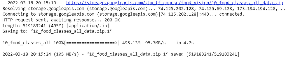
And now we'll turn the images into tensors datasets.
# Setup data inputs
import tensorflow as tf
IMG_SIZE = (224, 224)
train_data_10_classes_full = tf.keras.preprocessing.image_dataset_from_directory(train_dir,
                                                                                 label_mode="categorical",
                                                                                 image_size=IMG_SIZE)

# Note: this is the same test dataset we've been using for the previous modelling experiments
test_data = tf.keras.preprocessing.image_dataset_from_directory(test_dir,
                                                                label_mode="categorical",
                                                                image_size=IMG_SIZE)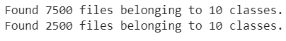
This is looking good. We've got 10x more images in of the training classes to work with.
The test dataset is the same we've been using for our previous experiments.
Let's evaluate
# Evaluate model (this is the fine-tuned 10 percent of data version)
model_2.evaluate(test_data)
Now we'll revert the model back to the saved weights.
# Load model from checkpoint, that way we can fine-tune from the same stage the 10 percent data model was fine-tuned from
model_2.load_weights(checkpoint_path) # revert model back to saved weights
Let's compile the model
# Compile
model_2.compile(loss="categorical_crossentropy",
                optimizer=tf.keras.optimizers.Adam(lr=0.0001), # divide learning rate by 10 for fine-tuning
                metrics=["accuracy"])
Time to fine-tune on all of the data!
# Continue to train and fine-tune the model to our data
fine_tune_epochs = initial_epochs + 5

history_fine_10_classes_full = model_2.fit(train_data_10_classes_full,
                                           epochs=fine_tune_epochs,
                                           initial_epoch=history_10_percent_data_aug.epoch[-1],
                                           validation_data=test_data,
                                           validation_steps=int(0.25 * len(test_data)),
                                           callbacks=[create_tensorboard_callback("transfer_learning", "full_10_classes_fine_tune_last_10")])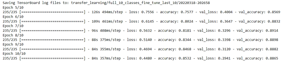
It looks like fine-tuning with all of the data has given our model a boost, how do the training curves look?
# How did fine-tuning go with more data?
compare_historys(original_history=history_10_percent_data_aug,
                 new_history=history_fine_10_classes_full,
                 initial_epochs=5)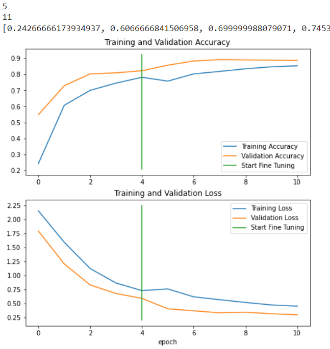
Looks like that extra data helped! Those curves are looking great. And if we trained for longer, they might even keep improving.