Computer Vision and Convolutional Neural Networks(CNN) with TensorFlow(Part 1)

Convolutional Neural Networks(CNN) is used for computer vision, which is detecting patterns of the visual data. For example,

If we want to classify whether a picture of food is pizza or bread.
We can detect some specific objects through a security camera.

In this blog, we would be going to learn how to build CNN to detect a visual object.

Get Data

Prepare data is the most important part of any deep learning project, we are going to work from the Food-101 dataset, a collection of 101 different categories of 101,000 (1000 images per category) real-world images of food dishes, to simplify the scenario we would choose two of the categories, pizza, and steak to build a binary classifier. we are thankful to Daniel Bourke to prepare data for pizza and steak only.

Import the Data

First, we need to import the data from the storage

import zipfile

# Download zip file of pizza_steak images
!wget https://storage.googleapis.com/ztm_tf_course/food_vision/pizza_steak.zip 

# Unzip the downloaded file
zip_ref = zipfile.ZipFile("pizza_steak.zip", "r")
zip_ref.extractall()
zip_ref.close()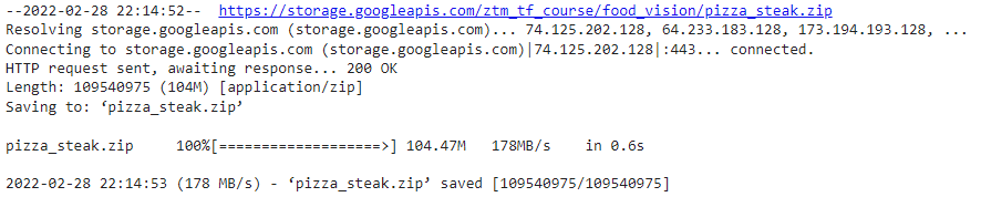

Inspect the Data

A very crucial step at the beginning of a machine learning project is to inspect the pattern and visualize the data. Let's inspect whatever data that we have just downloaded.

!ls pizza_steak

!ls pizza_steak/train/

!ls pizza_steak/train/steak/

-----

There are many images, now we need to find out how many images are there for train and test.

import os

# Walk through pizza_steak directory and list number of files
for dirpath, dirnames, filenames in os.walk("pizza_steak"):
  print(f"There are {len(dirnames)} directories and {len(filenames)} images in '{dirpath}'.")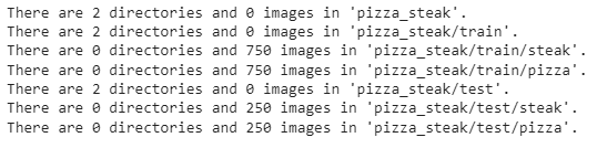

Get the class names (programmatically, this is much more helpful with a longer list of classes

import pathlib
import numpy as np
data_dir = pathlib.Path("pizza_steak/train/") # turn our training path into a Python path
class_names = np.array(sorted([item.name for item in data_dir.glob('*')])) # created a list of class_names from the subdirectories
print(class_names)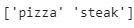

So, we have 750 training images and 250 test images of pizza and steak. Now we have to create a function to visualize the random images

# View an image
import matplotlib.pyplot as plt
import matplotlib.image as mpimg
import random

def view_random_image(target_dir, target_class):
  # Setup target directory (we'll view images from here)
  target_folder = target_dir+target_class

  # Get a random image path
  random_image = random.sample(os.listdir(target_folder), 1)

  # Read in the image and plot it using matplotlib
  img = mpimg.imread(target_folder + "/" + random_image[0])
  plt.imshow(img)
  plt.title(target_class)
  plt.axis("off");

  print(f"Image shape: {img.shape}") # show the shape of the image

  return img

Using this function let's try to visualize an image using target class(steak/pizza)

# View a random image from the training dataset
img = view_random_image(target_dir="pizza_steak/train/",
                        target_class="steak")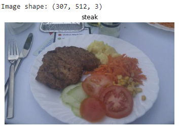


img = view_random_image(target_dir="pizza_steak/train/",
                        target_class="pizza")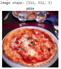

We can try out more results to get data. After getting more results we can get an idea of what we are working with. Now let's see the image in form of a big array/tensor and view the image shape.

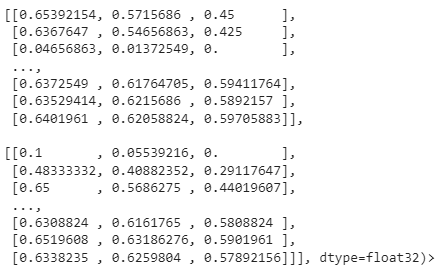
# View the img (actually just a big array/tensor) and shape((width, height, colour channels)
img, img.shape

-----

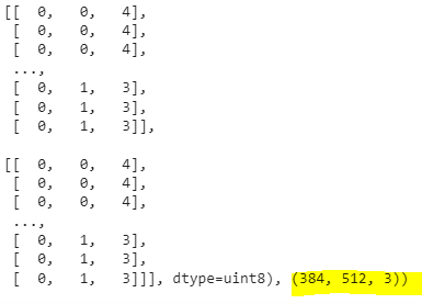
Now look at the image shape, it's in a form of with, Height, and Color Channels. We can notice all the values of the image array between 0 and 255. This is because that's the possible range of red, green, and blue values. So when we build a model to differentiate between our images of pizza and steak, it will be finding patterns in these different pixel values which determine what each class looks like.

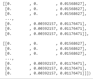
As we discuss before machine learning models prefer values between 0 and 1, one of the most common preprocessing steps for working with images is to scale the pixel value that is divided by 255.

# Get all the pixel values between 0 & 1
img/255.

-----

The architecture of a convolutional neural network(typical)

Why Typical? convolutional neural network deep learning network can be created in many different ways, we would discuss here the more traditional way of convolutional neural network(CNN).

Hyperparameter/Layer type What does it do? Typical values

Input image(s) Discover patterns of target image Photo or Video

Input layer Take a target image and input_shape = [batch_size,

preprocess image_height, image_width,

color_channels]

Convolution layer Extracts/learns the most Multiple, can create with

important features from target tf.keras.layers.ConvXD

images. (X can be multiple values)

Hidden activation Adds non-linearity to learned Usually ReLU

features (non-straight lines) (tf.keras.activations.relu)

Pooling layer Reduces the dimensionality of Average

learned image features (t f.keras.layers.AvgPool2D)

Max

(tf.keras.layers.MaxPool2D)

Fully connected layer Further refines learned features tf.keras.layers.Dense

from convolution layers

Output layer Takes learned features and output_shape =

outputs them in shape of target [number_of_classes]

labels.

Output activation Adds non-linearities to output tf.keras.activations.sigmoid

layer (binary classification) or

tf.keras.activations.softmax

How it looks

Resource: The architecture we're using below is a scaled-down version of VGG-16, a convolutional neural network that came 2nd in the 2014 ImageNet classification competition.

Binary classification

We just went through a whirlwind of steps:

Become one with the data (visualize, visualize, visualize...)
Preprocess the data (prepare it for a model)
Create a model (start with a baseline)
Fit the model
Evaluate the model
Adjust different parameters and improve the model (try to beat your baseline)
Repeat until satisfied

Let's step through each.

Prepare Data

Let's prepare data for our convolutional neural network (CNN) experiments.

One of the most important steps for a machine learning project is creating a training and test sets. In our case, our data is already split into training and test sets. Another option here might be to create a validation set as well, but we'll leave that for now. For an image classification project, it's standard to have your data separated into train and test directories with subfolders in each class.

A batch is a small subset of the dataset a model looks at during training. For example, rather than looking at 10,000 images at one time and trying to figure out the patterns, a model might only look at 32 images at a time.

It does this for a couple of reasons:

10,000 images (or more) might not fit into the memory of your processor (GPU).
Trying to learn the patterns in 10,000 images in one hit could result in the model not being able to learn very well.

Why 32?

There are many different batch sizes you could use but 32 has proven to be very effective in many different use cases and is often the default for many data preprocessing functions.

To turn our data into batches, we'll first create an instance of ImageDataGenerator for each of our datasets.


import tensorflow as tf
from tensorflow.keras.preprocessing.image import ImageDataGenerator

# Set the seed
tf.random.set_seed(42)

# Preprocess data (get all of the pixel values between 1 and 0, also called scaling/normalization)
train_datagen = ImageDataGenerator(rescale=1/255.)
test_datagen = ImageDataGenerator(rescale=1/255.)

# Setup the train and test directories
train_dir = "pizza_steak/train/"
test_dir = "pizza_steak/test/"

# Import data from directories and turn it into batches
# Turn it into batches
train_data = train_datagen.flow_from_directory(directory=train_dir,
                                               target_size=(224, 224),
                                               class_mode='binary',
                                               batch_size=32)

test_data = test_datagen.flow_from_directory(directory=test_dir,
                                             target_size=(224, 224),
                                             class_mode='binary',
                                             batch_size=32)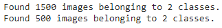

Looks like our training dataset has 1500 images belonging to 2 classes (pizza and steak) and our test dataset has 500 images also belonging to 2 classes.

Some things to here:

Due to how our directories are structured, the classes get inferred by the subdirectory names in train_dir and test_dir.
The target_size parameter defines the input size of our images in (height, width) format.
The class_mode value of 'binary' defines our classification problem type. If we had more than two classes, we would use 'categorical'.
The batch_size defines how many images will be in each batch, we've used 32 which is the same as the default.

We can take a look at our batched images and labels by inspecting the train_data object.


# Get a sample of the training data batch 
images, labels = train_data.next() # get the 'next' batch of images/labels
len(images), len(labels)

it seems our images and labels are in batches of 32.

How about the labels?

# View the first batch of labels
labels

Due to the class_mode parameter being 'binary' our labels are either 0 (pizza) or 1 (steak).

Create Model

A simple heuristic for computer vision models is to use the model architecture which is performing best on ImageNet (a large collection of diverse images to benchmark different computer vision models). However, to begin with, it's good to build a smaller model to acquire a baseline result that you try to improve upon. Let's create a small version of the model to acquire a baseline result and try to improve upon it.

# Make the creating of our model a little easier
from tensorflow.keras.optimizers import Adam
from tensorflow.keras.layers import Dense, Flatten, Conv2D, MaxPool2D, Activation
from tensorflow.keras import Sequential

# Create the model (this can be our baseline, a 3 layer Convolutional Neural Network)
model_1 = Sequential([
  Conv2D(filters=10, 
         kernel_size=3, 
         strides=1,
         padding='valid',
         activation='relu', 
         input_shape=(224, 224, 3)), # input layer (specify input shape)
  Conv2D(10, 3, activation='relu'),
  Conv2D(10, 3, activation='relu'),
  Flatten(),
  Dense(1, activation='sigmoid') # output layer (specify output shape)
])

Let's define the components of the Conv2D layer

The "2D" means our inputs are two-dimensional (height and width), even though they have 3 color channels, the convolutions are run on each channel individually.
filters - these are the number of "feature extractors" that will be moving over our images.
kernel_size - the size of our filters, for example, a kernel_size of (3, 3) (or just 3) will mean each filter will have the size 3x3, meaning it will look at a space of 3x3 pixels each time. The smaller the kernel, the more fine-grained features it will extract.
stride - the number of pixels a filter will move across as it covers the image. Astride of 1 means, the filter moves across each pixel 1 by 1. Astride of 2 means, it moves 2 pixels at a time.
padding - this can be either 'same' or 'valid', 'same' adds zeros the to outside of the image so the resulting output of the convolutional layer is the same as the input, whereas 'valid' (default) cuts off excess pixels where the filter doesn't fit (e.g. 224 pixels wide divided by a kernel size of 3 (224/3 = 74.6) means a single pixel will get cut off the end.

Resources:

CNN Explainer Webpage - a great visual overview of many of the concepts we're replicating here with code.
A guide to convolutional arithmetic for deep learning - a phenomenal introduction to the math going on behind the scenes of a convolutional neural network.
For a great explanation of padding, see this Stack Overflow answer.

Compile and Fit Model

# Compile the model
model_1.compile(loss='binary_crossentropy',
                optimizer=Adam(),
                metrics=['accuracy'])
# Fit the model
history_1 = model_1.fit(train_data,
                        epochs=5,
                        steps_per_epoch=len(train_data),
                        validation_data=test_data,
                        validation_steps=len(test_data))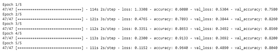

We'll notice two new parameters used here

steps_per_epoch - this is the number of batches a model will go through per epoch, in our case, we want our model to go through all batches so it's equal to the length of train_data (1500 images in batches of 32 = 1500/32 = ~47 steps)
validation_steps - same as above, except for the validation_data parameter (500 test images in batches of 32 = 500/32 = ~16 steps)

Let's create a function to investigate the model's training performance(separate accuracy and loss curves)

# Plot the validation and training data separately
def plot_loss_curves(history):
  """
  Returns separate loss curves for training and validation metrics.
  """ 
  loss = history.history['loss']
  val_loss = history.history['val_loss']

  accuracy = history.history['accuracy']
  val_accuracy = history.history['val_accuracy']

  epochs = range(len(history.history['loss']))

  # Plot loss
  plt.plot(epochs, loss, label='training_loss')
  plt.plot(epochs, val_loss, label='val_loss')
  plt.title('Loss')
  plt.xlabel('Epochs')
  plt.legend()

  # Plot accuracy
  plt.figure()
  plt.plot(epochs, accuracy, label='training_accuracy')
  plt.plot(epochs, val_accuracy, label='val_accuracy')
  plt.title('Accuracy')
  plt.xlabel('Epochs')
  plt.legend();

# Check out the loss curves of model_1
plot_loss_curves(history_1)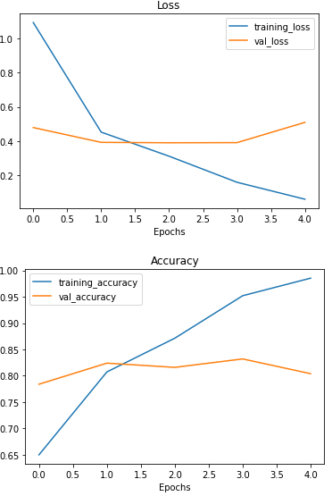

Repeat until satisified

After many iterations of the model experiment came up to dig into our bag of tricks and try another method of overfitting prevention, data augmentation.

Data augmentation is the process of altering our training data, leading to it having more diversity and in turn allowing our models to learn more generalizable patterns. Altering might mean adjusting the rotation of an image, flipping it, cropping it or something similar.

Doing this simulates the kind of data a model might be used on in the real world.

If we're building a pizza vs. steak application, not all of the images our users take might be in similar setups to our training data. Using data augmentation gives us another way to prevent overfitting and in turn make our model more generalizable. Let's data augmented test and train data.

# Create ImageDataGenerator training instance with data augmentation
train_datagen_augmented = ImageDataGenerator(rescale=1/255.,
                                             rotation_range=20, # rotate the image slightly between 0 and 20 degrees (note: this is an int not a float)
                                             shear_range=0.2, # shear the image
                                             zoom_range=0.2, # zoom into the image
                                             width_shift_range=0.2, # shift the image width ways
                                             height_shift_range=0.2, # shift the image height ways
                                             horizontal_flip=True) # flip the image on the horizontal axis

# Create ImageDataGenerator training instance without data augmentation
train_datagen = ImageDataGenerator(rescale=1/255.) 

# Create ImageDataGenerator test instance without data augmentation
test_datagen = ImageDataGenerator(rescale=1/255.)

# Import data and augment it from training directory
print("Augmented training images:")
train_data_augmented = train_datagen_augmented.flow_from_directory(train_dir,
                                                                   target_size=(224, 224),
                                                                   batch_size=32,
                                                                   class_mode='binary',
                                                                   shuffle=False) # Don't shuffle for demonstration purposes, usually a good thing to shuffle

# Create non-augmented data batches
print("Non-augmented training images:")
train_data = train_datagen.flow_from_directory(train_dir,
                                               target_size=(224, 224),
                                               batch_size=32,
                                               class_mode='binary',
                                               shuffle=False) # Don't shuffle for demonstration purposes

print("Unchanged test images:")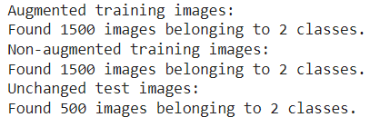

Let's visualize data augmentation, how about we see it?


# Get data batch samples
images, labels = train_data.next()
augmented_images, augmented_labels = train_data_augmented.next() # Note: labels aren't augmented, they stay the same

# Show original image and augmented image
random_number = random.randint(0, 32) # we're making batches of size 32, so we'll get a random instance
plt.imshow(images[random_number])
plt.title(f"Original image")
plt.axis(False)
plt.figure()
plt.imshow(augmented_images[random_number])
plt.title(f"Augmented image")
plt.axis(False);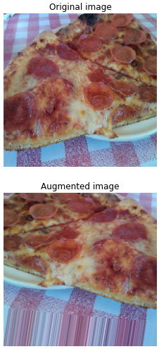

After going through a sample of original and augmented images, you can start to see some of the example transformations on the training images.

Notice how some of the augmented images look like slightly warped versions of the original image. This means our model will be forced to try and learn patterns in less-than-perfect images, which is often the case when using real-world images.

We need to try to create models until satisfy the result

Let's see what happens when we shuffle the augmented training data.


# Import data and augment it from directories
train_data_augmented_shuffled = train_datagen_augmented.flow_from_directory(train_dir,
                                                                            target_size=(224, 224),
                                                                            batch_size=32,
                                                                            class_mode='binary',
                                                                            shuffle=True) # Shuffle data (default)

Since we've already beaten our baseline, there are a few things we could try to continue to improve our model:

Increase the number of model layers (e.g. add more convolutional layers).
Increase the number of filters in each convolutional layer (e.g. from 10 to 32, 64, or 128, these numbers aren't set in stone either, they are usually found through trial and error).
Train for longer (more epochs).
Finding an ideal learning rate.
Get more data (give the model more opportunities to learn).

Adjusting each of these settings (except for the last two) during model development is usually referred to as hyperparameter tuning.

You can think of hyperparameter tuning as similar to adjusting the settings on your oven to cook your favorite dish. Although your oven does most of the cooking for you, you can help it by tweaking the dials. Here is our final model

# Create a CNN model (same as Tiny VGG but for binary classification - https://poloclub.github.io/cnn-explainer/ )
model_final = Sequential([
  Conv2D(10, 3, activation='relu', input_shape=(224, 224, 3)), # same input shape as our images
  Conv2D(10, 3, activation='relu'),
  MaxPool2D(),
  Conv2D(10, 3, activation='relu'),
  Conv2D(10, 3, activation='relu'),
  MaxPool2D(),
  Flatten(),
  Dense(1, activation='sigmoid')
])

# Compile the model
model_final.compile(loss="binary_crossentropy",
                optimizer=tf.keras.optimizers.Adam(),
                metrics=["accuracy"])

# Fit the model
history_final = model_final.fit(train_data_augmented_shuffled,
                        epochs=5,
                        steps_per_epoch=len(train_data_augmented_shuffled),
                        validation_data=test_data,
                        validation_steps=len(test_data))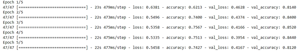

Now let's check out our TinyVGG model's performance.

plot_loss_curves(history_final)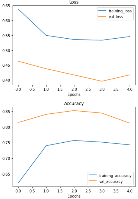

Now our training curves are looking good, however, we can improve more if we trained it a little longer.

Prediction Our Trained Model

What good is a trained model if you can't make predictions with it?

To really test it out, we'll upload a couple of our own images and see how the model goes, you can test with your own image as well.

The first test image we're going to use is a delicious steak.

# View our example image
!wget https://raw.githubusercontent.com/sumitdeyonline/machinelearning/main/03-steak.jpeg 
steak = mpimg.imread("03-steak.jpeg")
plt.imshow(steak)
plt.axis(False);

Check the shape of the image

# Check the shape of our image
steak.shape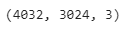

Since our model takes in images of shapes (224, 224, 3), we've got to reshape our custom image to use it with our model.

To do so, we can import and decode our image using tf.io.read_file (for reading files) and tf.image (for resizing our image and turning it into a tensor). Let's create a function to convert the image preparation.

# Create a function to import an image and resize it to be able to be used with our model
def load_and_prep_image(filename, img_shape=224):
  """
  Reads an image from filename, turns it into a tensor
  and reshapes it to (img_shape, img_shape, colour_channel).
  """
  # Read in target file (an image)
  img = tf.io.read_file(filename)

  # Decode the read file into a tensor & ensure 3 colour channels 
  # (our model is trained on images with 3 colour channels and sometimes images have 4 colour channels)
  img = tf.image.decode_image(img, channels=3)

  # Resize the image (to the same size our model was trained on)
  img = tf.image.resize(img, size = [img_shape, img_shape])

  # Rescale the image (get all values between 0 and 1)
  img = img/255.
  return img

Now we've got a function to load our custom image, let's load it in.

# Load in and preprocess our custom image
steak = load_and_prep_image("03-steak.jpeg")
steak

----

There's one more problem. Although our image is in the same shape as the images our model has been trained on, we're still missing a dimension. Remember how our model was trained in batches? Well, the batch size becomes the first dimension.

So in reality, our model was trained on data in the shape of (batch_size, 224, 224, 3).

We can fix this by adding an extra to our custom image tensor using tf.expand_dims.

# Add an extra axis
print(f"Shape before new dimension: {steak.shape}")
steak = tf.expand_dims(steak, axis=0) # add an extra dimension at axis 0
#steak = steak[tf.newaxis, ...] # alternative to the above, '...' is short for 'every other dimension'
print(f"Shape after new dimension: {steak.shape}")
steak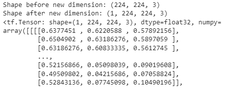

----

the predictions come out in prediction probability form. In other words, this means how likely the image is to be one class or another.

Since we're working with a binary classification problem, if the prediction probability is over 0.5, according to the model, the prediction is most likely to be a positive class (class 1).

And if the prediction probability is under 0.5, according to the model, the predicted class is most likely to be the negative class (class 0)

Let's create a function that would make a prediction of the input image using the trained model and plot the image with the predicted class as the title.

def pred_and_plot(model, filename, class_names):
  """
  Imports an image located at filename, makes a prediction on it with
  a trained model and plots the image with the predicted class as the title.
  """
  # Import the target image and preprocess it
  img = load_and_prep_image(filename)

  # Make a prediction
  pred = model.predict(tf.expand_dims(img, axis=0))

  # Get the predicted class
  pred_class = class_names[int(tf.round(pred)[0][0])]

  # Plot the image and predicted class
  plt.imshow(img)
  plt.title(f"Prediction: {pred_class}")
  plt.axis(False);

Finally, making a test of our custom image with prediction

# Test our model on a custom image
pred_and_plot(model_final, "03-steak.jpeg", class_names)

Wow.. Our prediction is right, our model starts working. You can start predicting more images using pred_and_plot function. Please try yourself.

In the next part, we would discuss about Multi-class classification with Convolutional Neural Networks(CNN) (Part 2), stay tuned.