- Sumit Dey
- Apr 11, 2022
- 3 min read
There are many ways to build machine learning models and we have to do many experiments with those models, it is very impotent to save models in different stages of experiments. Today we would discuss more how we can start an experiment and save the model for future reference. Let's create a feature extraction model and save the whole model as a file.
Use TensorFlow Datasets to Download Data
What are TensorFlow Datasets?
Load data already in Tensors
Practice on well-established datasets
Experiment with different data loading techniques.
Experiment with new TensorFlow features quickly (such as mixed precision training)
Why not use TensorFlow Datasets?
The datasets are static (they don't change as your real-world datasets would)
Might not be suited for your particular problem (but great for experimenting)
To find all of the available datasets in TensorFlow Datasets, you can use the list_builders() method. It looks like the dataset we're after is available (note there are plenty more available but we're on Food101). To get access to the Food101 dataset from the TFDS, we can use the tfds.load() method. In particular, we'll have to pass it a few parameters to let it know what we're after:
name (str) : the target dataset (e.g. "food101")
split (list, optional) : what splits of the dataset we're after (e.g. ["train", "validation"])
the split parameter is quite tricky. See the documentation for more.
shuffle_files (bool) : whether or not to shuffle the files on download, defaults to False
as_supervised (bool) : True to download data samples in tuple format ((data, label)) or False for dictionary format
with_info (bool) : True to download dataset metadata (labels, number of samples, etc.)
# Get TensorFlow Datasets
import tensorflow_datasets as tfds
# Load in the data (takes about 5-6 minutes in Google Colab)
(train_data, test_data), ds_info = tfds.load(name="food101", # target dataset to get from TFDS
                                             split=["train", "validation"], # what splits of data should we get? note: not all datasets have train, valid, test
                                             shuffle_files=True, # shuffle files on download?
                                             as_supervised=True, # download data in tuple format (sample, label), e.g. (image, label)
                                             with_info=True) # include dataset metadata? if so, tfds.load() returns tuple (data, ds_info)
After a few minutes of downloading, we've now got access to the entire Food101 dataset (in tensor format) ready for modeling. Now let's get a little information from our dataset, starting with the class names. Getting class names from a TensorFlow Datasets dataset requires downloading the "dataset_info" variable (by using the as_supervised=True parameter in the tfds.load() method, note: this will only work for supervised datasets in TFDS). We can access the class names of a particular dataset using the dataset_info.features attribute and accessing the names attribute of the "label" key.
# Get class names
class_names = ds_info.features["label"].names
class_names[:10]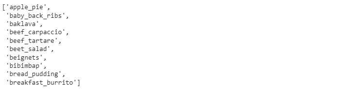
Now we are creating the model
import tensorflow as tf
from tensorflow.keras import layers
from tensorflow.keras.layers.experimental import preprocessing

# Create base model
input_shape = (224, 224, 3)
base_model = tf.keras.applications.EfficientNetB0(include_top=False)
base_model.trainable = False # freeze base model layers

# Create Functional model
inputs = layers.Input(shape=input_shape, name="input_layer", dtype=tf.float16)
# Note: EfficientNetBX models have rescaling built-in but if your model didn't you could have a layer like below
# x = preprocessing.Rescaling(1./255)(x)
x = base_model(inputs, training=False) # set base_model to inference mode only
x = layers.GlobalAveragePooling2D(name="pooling_layer")(x)
x = layers.Dense(len(class_names))(x) # want one output neuron per class
# Separate activation of output layer so we can output float32 activations
outputs = layers.Activation("softmax", dtype=tf.float32, name="softmax_float32")(x)
model = tf.keras.Model(inputs, outputs)

# Compile the model
model.compile(loss="sparse_categorical_crossentropy", # Use sparse_categorical_crossentropy when labels are *not* one-hot
              optimizer=tf.keras.optimizers.Adam(),
              metrics=["accuracy"])
Get the model summary
# Get the model summary
model.summary()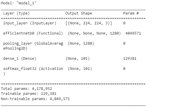
Save the whole model to file
We can also save the whole model using the save() method. Since our model is quite large, you might want to save it to Google Drive (if you're using Google Colab) so you can load it in for use later.
## Saving model to Google Drive
# Create save path to drive
save_dir = "drive/MyDrive/tensorflow_blog/food_vision/07_efficientnetb0_feature_extract_model_mixed_precision/"
# os.makedirs(save_dir) # Make directory if it doesn't exist

# Save model
model.save(save_dir)
We can also save it directly to our Google Colab instance.
# Save model locally (if you're using Google Colab, your saved model will Colab instance terminates)
save_dir = "07_efficientnetb0_feature_extract_model_mixed_precision"
model.save(save_dir)
And again, we can check whether or not our model is saved correctly by loading it.
# Load model previously saved above
loaded_saved_model = tf.keras.models.load_model(save_dir)
Get the model summary
# Get the model summary
loaded_saved_model.summary()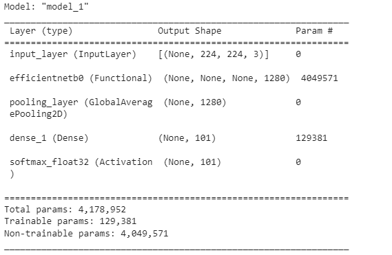
Both the models seem the same.


