Transfer Learning with TensorFlow(Part 1)

In our previous blogs, we've built a bunch of convolutional neural networks from scratch and they all seem to be learning, however, there is still plenty of room for improvement. To improve our model(s), we could spend a while trying different configurations, adding more layers, changing the learning rate, adjusting the number of neurons per layer, and more, doing all this is very time-consuming.

We're lucky that there's a technique to save time, it is called transfer learning, in other words, taking the patterns (also called weights) another model has learned from another problem and using them for our own problem.

Here is the befit of using transfer learning

Can leverage an existing neural network architecture proven to work on problems similar to our own.
Can leverage a working neural network architecture that has already learned patterns on similar data to our own. This often results in achieving great results with fewer custom data.

What this means is, instead of hand-crafting our own neural network architectures or building them from scratch, we can utilize models which have worked for others.

And instead of training our own models from scratch on our own datasets, we can take the patterns a model has learned from datasets such as ImageNet (millions of images of different objects) and use them as the foundation of our own. Doing this often leads to getting great results with less data.

Transfer learning with TensorFlow Hub

For many of the problems you'll want to use deep learning for, chances are, a working model already exists. And the good news is, you can access many of them on TensorFlow Hub.

TensorFlow Hub is a repository for existing model components. It makes it so you can import and use a fully trained model with as little as a URL. e could get much of the same results (or better) than our best model has gotten so far with only 10% of the original data, in other words, 10x fewer data.

Transfer learning often allows you to get great results with less data. et's download a subset of the data we've been using, namely 10% of the training data from the 10_food_classes dataset and use it to train a food image classifier.

Let's download the data and execute it with the existing model

Download data

Let's get the data from the Food-101 dataset. we would work with 10 percent of the data.

# Get data (10% of labels)
import zipfile

# Download data
!wget https://storage.googleapis.com/ztm_tf_course/food_vision/10_food_classes_10_percent.zip

# Unzip the downloaded file
zip_ref = zipfile.ZipFile("10_food_classes_10_percent.zip", "r")
zip_ref.extractall()
zip_ref.close()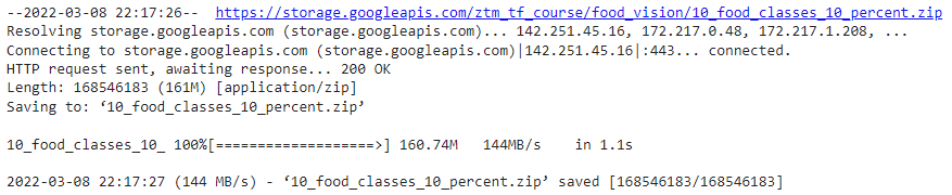

Let's find out how many images are in the folder

# How many images in each folder?
import os

# Walk through 10 percent data directory and list number of files
for dirpath, dirnames, filenames in os.walk("10_food_classes_10_percent"):
  print(f"There are {len(dirnames)} directories and {len(filenames)} images in '{dirpath}'.")

Notice how each of the training directories now has 75 images rather than 750 images. This is key to demonstrating how well transfer learning can perform with less labeled images.

The test directories still have the same amount of images. This means we'll be training on less data but evaluating our models on the same amount of test data.

Preparing the data

Now we've downloaded the data, let's use the ImageDataGenerator class along with the flow_from_directory method to load in our images.

# Setup data inputs
from tensorflow.keras.preprocessing.image import ImageDataGenerator

IMAGE_SHAPE = (224, 224)
BATCH_SIZE = 32

train_dir = "10_food_classes_10_percent/train/"
test_dir = "10_food_classes_10_percent/test/"

train_datagen = ImageDataGenerator(rescale=1/255.)
test_datagen = ImageDataGenerator(rescale=1/255.)

print("Training images:")
train_data_10_percent = train_datagen.flow_from_directory(train_dir,
                                               target_size=IMAGE_SHAPE,
                                               batch_size=BATCH_SIZE,
                                               class_mode="categorical")

print("Testing images:")
test_data = train_datagen.flow_from_directory(test_dir,
                                              target_size=IMAGE_SHAPE,
                                              batch_size=BATCH_SIZE,
                                              class_mode="categorical")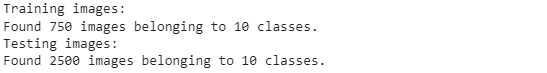

Loading in the data we can see we've got 750 images in the training dataset belonging to 10 classes (75 per class) and 2500 images in the test set belonging to 10 classes (250 per class).

Setting up callbacks

What are callbacks? Callbacks are extra functionality you can add to your models to be performed during or after training. Some of the most popular callbacks include:

Experiment tracking with TensorBoard - log the performance of multiple models and then view and compare these models in a visual way on TensorBoard (a dashboard for inspecting neural network parameters). Helpful to compare the results of different models on your data.
Model checkpointing - save your model as it trains so you can stop training if needed and come back to continue off where you left. Helpful if training takes a long time and can't be done in one sitting.
Early stopping - leave your model training for an arbitrary amount of time and have it stop training automatically when it ceases to improve. Helpful when you've got a large dataset and don't know how long training will take.

The TensorBoard callback can be accessed using tf.keras.callbacks.TensorBoard().

Its main functionality is saving a model's training performance metrics to a specified log_dir.

By default, logs are recorded every epoch using the update_freq='epoch' parameter. This is a good default since tracking model performance too often can slow down model training.

To track our modeling experiments using TensorBoard, let's create a function that creates a TensorBoard callback for us.

# Create tensorboard callback (functionized because need to create a new one for each model)
import datetime
def create_tensorboard_callback(dir_name, experiment_name):
  log_dir = dir_name + "/" + experiment_name + "/" + datetime.datetime.now().strftime("%Y%m%d-%H%M%S")
  tensorboard_callback = tf.keras.callbacks.TensorBoard(
      log_dir=log_dir
  )
  print(f"Saving TensorBoard log files to: {log_dir}")
  return tensorboard_callback

Because you're likely to run multiple experiments, it's a good idea to be able to track them in some way. In our case, our function saves a model's performance logs to a directory named [dir_name]/[experiment_name]/[current_timestamp], where:

dir_name is the overall logs directory
experiment_name is the particular experiment
current_timestamp is the time the experiment started based on Python's datetime.datetime().now()

Creating models using TensorFlow Hub

In the past, we've used TensorFlow to create our own model layer by layer from scratch.

Now we're going to do a similar process, except the majority of our model's layers are going to come from TensorFlow Hub.

In fact, we're going to use two models from TensorFlow Hub:

ResNetV2 - a state-of-the-art computer vision model architecture from 2016.
EfficientNet - a state-of-the-art computer vision architecture from 2019.

State of the art means that at some point, both of these models have achieved the lowest error rate on ImageNet (ILSVRC-2012-CLS), the gold standard of computer vision benchmarks.

How do you find the TensorFlow Hub? Here are the steps

Go to tfhub.dev.
Choose your problem domain, e.g. "Image" (we're using food images).
Select your TF version, which in our case is TF2.
Remove all "Problem domanin" filters except for the problem you're working on.
The models listed are all models which could potentially be used for your problem.

To find our models, let's narrow down our search using the Architecture tab.

Select the Architecture tab on TensorFlow Hub and you'll see a dropdown menu of architecture names appear.
- The rule of thumb here is generally, names with larger numbers mean better performing models. For example, EfficientNetB4 performs better than EfficientNetB0.
  - However, the tradeoff with larger numbers can mean they take longer to compute.

This is where the different types of transfer learning come into play, as is, feature extraction and fine-tuning.

1. "As is" transfer learning is when you take a pre-trained model as it is and apply it to your task without any changes. For example, many computer vision models are pre-trained on the ImageNet dataset which contains 1000 different classes of images. This means passing a single image to this model will produce 1000 different prediction probability values (1 for each class).

This is helpful if you have 1000 classes of the image you'd like to classify and they're all the same as the ImageNet classes, however, it's not helpful if you want to classify only a small subset of classes (such as 10 different kinds of food). Model's with "/classification" in their name on TensorFlow Hub provide this kind of functionality.

2. Feature extraction transfer learning is when you take the underlying patterns (also called weights) a pre-trained model has learned and adjust its outputs to be more suited to your problem.

For example, say the pre-trained model you were using had 236 different layers (EfficientNetB0 has 236 layers), but the top layer outputs 1000 classes because it was pre-trained on ImageNet. To adjust this to your own problem, you might remove the original activation layer and replace it with your own but with the right number of output classes. The important part here is that only the top few layers become trainable, the rest remain frozen.
- This way all the underlying patterns remain in the rest of the layers and you can utilize them for your own problem. This kind of transfer learning is very helpful when your data is similar to the data a model has been pre-trained on.

3. Fine-tuning transfer learning is when you take the underlying patterns (also called weights) of a pre-trained model and adjust (fine-tune) them to your own problem.

This usually means training some, many, or all of the layers in the pre-trained model. This is useful when you've got a large dataset (e.g. 100+ images per class) where your data is slightly different from the data the original model was trained on.

A common workflow is to "freeze" all of the learned patterns in the bottom layers of a pre-trained model so they're untrainable. And then train the top 2-3 layers of so the pre-trained model can adjust its outputs to your custom data (feature extraction).

After you've trained the top 2-3 layers, you can then gradually "unfreeze" more and more layers and run the training process on your own data to further fine-tune the pre-trained model.

Now we'll get the feature vector URLs of two common computer vision architectures, EfficientNetB0 (2019) and ResNetV250 (2016) from TensorFlow Hub using the steps above.

We're getting both of these because we're going to compare them to see which performs better on our data.

Comparing different model architecture performances on the same data is a very common practice. The simple reason is that you want to know which model performs best for your problem.

# Resnet 50 V2 feature vector
resnet_url = "https://tfhub.dev/google/imagenet/resnet_v2_50/feature_vector/4"

# Original: EfficientNetB0 feature vector (version 1)
efficientnet_url = "https://tfhub.dev/tensorflow/efficientnet/b0/feature-vector/1"

# # New: EfficientNetB0 feature vector (version 2)
# efficientnet_url = "https://tfhub.dev/google/imagenet/efficientnet_v2_imagenet1k_b0/feature_vector/2"

These URLs link to a saved pre-trained model on TensorFlow Hub. When we use them in our model, the model will automatically be downloaded for us to use. To do this, we can use the KerasLayer() model inside the TensorFlow hub library.

Since we're going to be comparing two models, to save ourselves code, we'll create a function create_model(). This function will take a model's TensorFlow Hub URL, instantiate a Keras Sequential model with the appropriate number of output layers and return the model.

import tensorflow as tf
import tensorflow_hub as hub
from tensorflow.keras import layers  
def create_model(model_url, num_classes=10):
  """Takes a TensorFlow Hub URL and creates a Keras Sequential model with it.
  
  Args:
    model_url (str): A TensorFlow Hub feature extraction URL.
    num_classes (int): Number of output neurons in output layer,
      should be equal to number of target classes, default 10.

  Returns:
    An uncompiled Keras Sequential model with model_url as feature
    extractor layer and Dense output layer with num_classes outputs.
  """
  # Download the pretrained model and save it as a Keras layer
  feature_extractor_layer = hub.KerasLayer(model_url,
                                           trainable=False, # freeze the underlying patterns
                                           name='feature_extraction_layer',
                                           input_shape=IMAGE_SHAPE+(3,)) # define the input image shape
  
  # Create our own model
  model = tf.keras.Sequential([
    feature_extractor_layer, # use the feature extraction layer as the base
    layers.Dense(num_classes, activation='softmax', name='output_layer') # create our own output layer      
  ])

  return model

Now we've got a function for creating a model, we'll use it to first create a model using the ResNetV250 architecture as our feature extraction layer.

Once the model is instantiated, we'll compile it using categorical_crossentropy as our loss function, the Adam optimizer, and accuracy as our metric.

# Create model
resnet_model = create_model(resnet_url, num_classes=train_data_10_percent.num_classes)

# Compile
resnet_model.compile(loss='categorical_crossentropy',
                     optimizer=tf.keras.optimizers.Adam(),
                     metrics=['accuracy'])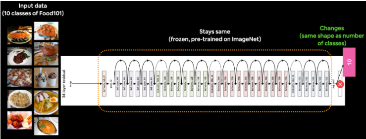

Now we need to fit the model. We've got the training data ready in train_data_10_percent as well as the test data saved as test_data. But before we call the fit function, there's one more thing we're going to add, a callback. More specifically, a TensorBoard callback so we can track the performance of our model on TensorBoard. We can add a callback to our model by using the callbacks parameter in the fit function. In our case, we'll pass the callbacks parameter the create_tensorboard_callback() we created earlier with some specific inputs so we know what experiments we're running.

Let's keep the experiment short and train for 5 epochs

# Fit the model
resnet_history = resnet_model.fit(train_data_10_percent,
                                  epochs=5,
                                  steps_per_epoch=len(train_data_10_percent),
                                  validation_data=test_data,
                                  validation_steps=len(test_data),
                                  # Add TensorBoard callback to model (callbacks parameter takes a list)
                                  callbacks=[create_tensorboard_callback(dir_name="tensorflow_hub", # save experiment logs here
                                                                         experiment_name="resnet50V2")]) # name of log files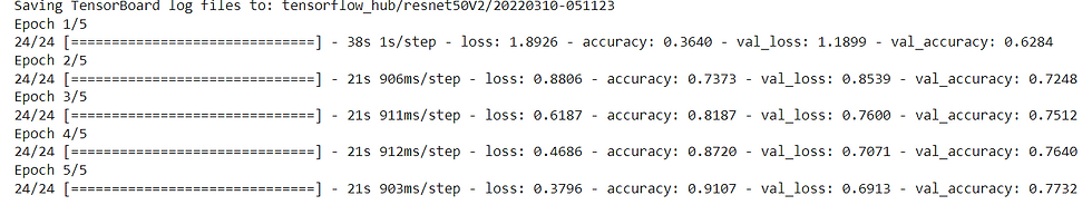

It seems that after only 5 epochs, the ResNetV250 feature extraction model was able to blow any of the architectures we made out of the water, achieving around 90% accuracy on the training set and nearly 80% accuracy on the test set...with only 10 percent of the training images!

That goes to show the power of transfer learning. And it's one of the main reasons whenever you're trying to model your own datasets, you should look into what pre-trained models already exist.

Let's check out our model's training curves using our plot_loss_curves function.

# If you wanted to, you could really turn this into a helper function to load in with a helper.py script...
import matplotlib.pyplot as plt

# Plot the validation and training data separately
def plot_loss_curves(history):
  """
  Returns separate loss curves for training and validation metrics.
  """ 
  loss = history.history['loss']
  val_loss = history.history['val_loss']

  accuracy = history.history['accuracy']
  val_accuracy = history.history['val_accuracy']

  epochs = range(len(history.history['loss']))

  # Plot loss
  plt.plot(epochs, loss, label='training_loss')
  plt.plot(epochs, val_loss, label='val_loss')
  plt.title('Loss')
  plt.xlabel('Epochs')
  plt.legend()

  # Plot accuracy
  plt.figure()
  plt.plot(epochs, accuracy, label='training_accuracy')
  plt.plot(epochs, val_accuracy, label='val_accuracy')
  plt.title('Accuracy')
  plt.xlabel('Epochs')
  plt.legend();

plot_loss_curves(resnet_history)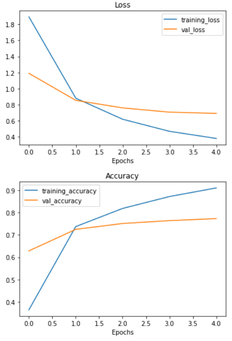

Okay, we've trained a ResNetV250 model, time to do the same with the EfficientNetB0 model. The setup will be the exact same as before, except for the model_url parameter in the create_model() function and the experiment_name parameter in the create_tensorboard_callback() function.

# Create model
efficientnet_model = create_model(model_url=efficientnet_url, # use EfficientNetB0 TensorFlow Hub URL
                                  num_classes=train_data_10_percent.num_classes)

# Compile EfficientNet model
efficientnet_model.compile(loss='categorical_crossentropy',
                           optimizer=tf.keras.optimizers.Adam(),
                           metrics=['accuracy'])

# Fit EfficientNet model 
efficientnet_history = efficientnet_model.fit(train_data_10_percent, # only use 10% of training data
                                              epochs=5, # train for 5 epochs
                                              steps_per_epoch=len(train_data_10_percent),
                                              validation_data=test_data,
                                              validation_steps=len(test_data),
                                              callbacks=[create_tensorboard_callback(dir_name="tensorflow_hub", 
                                                                                     # Track logs under different experiment name
                                                                                     experiment_name="efficientnetB0")])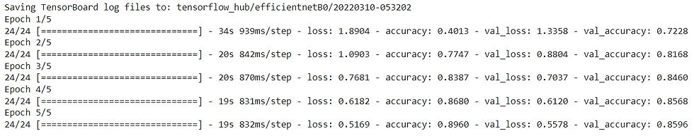

The EfficientNetB0 model does even better than the ResNetV250 model! Achieving over 85% accuracy on the test set...again with only 10% of the training data.

How cool is that? With a couple of lines of code, we're able to leverage state-of-the-art models and adjust them to our own use case.

plot_loss_curves(efficientnet_history)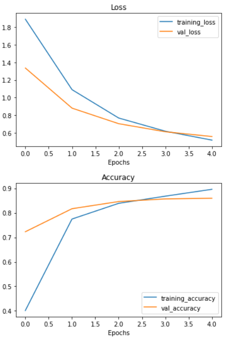

From the look of the EfficientNetB0 model's loss curves, it looks like if we kept training our model for longer, it might improve even further. Perhaps that's something you might want to predict?

Make a Prediction

Let's try the same image from the previous section and try to predict

# Create a function to import an image and resize it to be able to be used with our model
def load_and_prep_image(filename, img_shape=224):
  """
  Reads an image from filename, turns it into a tensor
  and reshapes it to (img_shape, img_shape, colour_channel).
  """
  # Read in target file (an image)
  img = tf.io.read_file(filename)

  # Decode the read file into a tensor & ensure 3 colour channels 
  # (our model is trained on images with 3 colour channels and sometimes images have 4 colour channels)
  img = tf.image.decode_image(img, channels=3)

  # Resize the image (to the same size our model was trained on)
  img = tf.image.resize(img, size = [img_shape, img_shape])

  # Rescale the image (get all values between 0 and 1)
  img = img/255.
  return img

# Adjust function to work with multi-class
def pred_and_plot(model, filename, class_names):
  """
  Imports an image located at filename, makes a prediction on it with
  a trained model and plots the image with the predicted class as the title.
  """
  # Import the target image and preprocess it
  img = load_and_prep_image(filename)

  # Make a prediction
  pred = model.predict(tf.expand_dims(img, axis=0))

  # Get the predicted class
  if len(pred[0]) > 1: # check for multi-class
    pred_class = class_names[pred.argmax()] # if more than one output, take the max
  else:
    pred_class = class_names[int(tf.round(pred)[0][0])] # if only one output, round

  # Plot the image and predicted class
  plt.imshow(img)
  plt.title(f"Prediction: {pred_class}")
  plt.axis(False);

class_names = ['chicken_curry', 'chicken_wings', 'fried_rice', 'grilled_salmon','hamburger', 'ice_cream', 'pizza', 'ramen', 'steak', 'sushi']

Let's try out the prediction again

pred_and_plot(efficientnet_model, "03-hamburgerandfries.jpeg", class_names)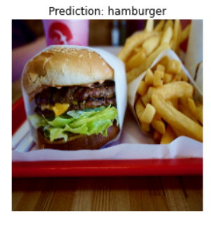

Wow!!! now the prediction is correct, it's "hamburger". In our custom model, it was predicted "steak", let's try more images

pred_and_plot(efficientnet_model, "03-sushi.jpeg", class_names)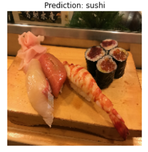

Again prediction is correct, it's "Sushi". In our custom model, it was predicted "ramen"

This is the power of transfer learning. We would discuss more transfer learning in my next Blogs. Stay Tuned.